How Transformers Work: A Plain Explanation
Let’s revisit transformers and try to figure out how they actually work — as usual, minimal math and no AI-generated filler. The author makes no claims to absolute truth and may occasionally get things slightly wrong.
1. Let’s Start Simple
Let’s refresh our memory on how recurrent networks worked — the ones that “loop back to themselves”. Hard not to think of Hegel’s Absolute Spirit, which travels a path of self-alienation only to return to itself — pure Hegelian recurrence.
How RNN Worked: Passing Notes Down the Line
Picture four colleagues sitting in a row. Each sees only one word and receives a note from the person on their left — a brief summary of everything before them. Their job: read their word, update the note, and pass it on.
The phrase: “the cat sat on the roof”
Person 1 🧑 sees the word “cat”. No note yet (they’re first). Writes on a sticky: “we’re talking about a cat” → passes right.
Person 2 🧑 sees “sat”, receives the sticky “we’re talking about a cat”. Erases, updates, passes: “cat sat” → right.
Person 3 🧑 sees “on”, receives the sticky, updates: “cat sat on…” → right.
Person 4 🧑 sees “roof”, updates: “cat sat on the roof”.
Each step depends on the previous one — information flows strictly sequentially through a single sticky (a hidden state vector).
What’s the Problem?
Of course, real neural network stickies contain no words — just numbers: a fixed vector of, say, 512 values. Think embeddings — a multidimensional semantic space (more on that here). Each person in the chain receives 512 numbers, sees their word, and writes 512 new numbers encoding the meaning of everything before. Not “cat sat”, but a single numerical representation — coordinates in semantic space encoding that we’re talking about a cat, that it’s doing something, and that it’s somewhere up high.
But the sticky has a fixed size. With short phrases it’s fine. But imagine a 50-word sentence: by word 40, the person receives a sticky that’s been erased and rewritten 39 times. Information about the first words has blurred out. The network literally forgets the beginning.
And speed. Person 2 can’t start until Person 1 passes the note. Person 3 waits for Person 2. Everyone queues up. Meanwhile GPUs are built for thousands of parallel operations — sequential processing like this is a poor fit.
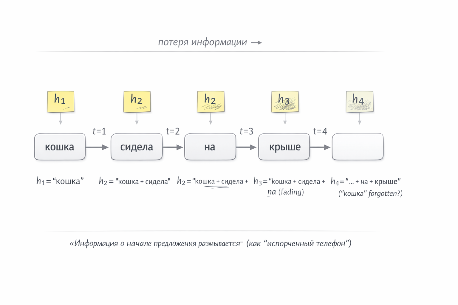
Fig. 1. How an RNN processes “the cat sat on the roof” — passing a sticky note down the chain
Transformer: Everyone Sees Everything
Now the transformer arrives, scrapping this scheme entirely. Instead of four people passing a note, imagine a round table: all four words are in front of the model simultaneously, and each can directly look at any other. The word “roof” doesn’t need to wait for information about “cat” to crawl through intermediate steps — it sees “cat” directly.
As a result:
- No information loss — every word has direct access to every other word, no intermediaries.
- Full parallelism — all words are processed simultaneously, keeping the GPU fully loaded.
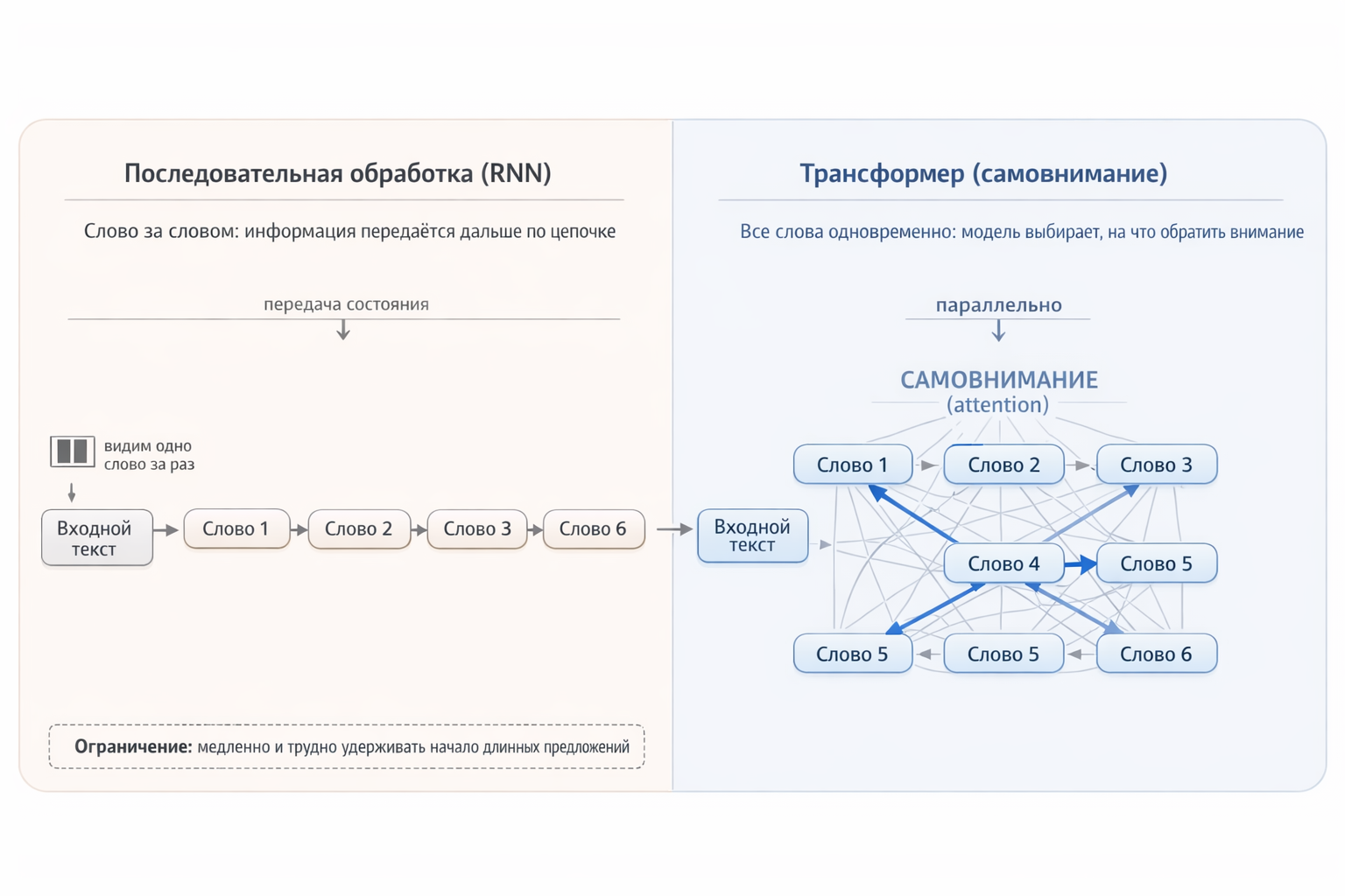
Fig. 2. Sequential processing vs. the transformer’s parallel “gaze”
2. Overall Architecture: Layer by Layer
A transformer is a stack of identical layers (typically 12 to 96+). Each layer contains two blocks:
- Self-Attention — already covered in the linked article above. Determines which words in a sentence relate to each other and how.
- Feed-Forward Network (FFN) — interesting. Processes each word individually, “enriching it” with knowledge. This is what we’ll dig into.
Words in the prompt pass through all layers bottom to top — and at each level the model builds a deeper understanding of the text. But what does “deeper understanding” actually mean? What can a model “understand”? We can’t even explain how we understand things — Ginzburg (Nobel laureate in physics) considered the phenomenon of consciousness one of physics’ key unsolved puzzles. On that note, the author’s obligatory erudition detour ends.
What Goes In and What Comes Out
The transformer receives text split into tokens (words or word pieces). Each token becomes a numerical vector — an embedding — of, say, 4096 numbers. This is the starting numerical representation of the word.
The output is an updated vector for each input token. To predict the next word, the last token’s vector (which encodes the meaning of the entire text) passes through a final linear layer and a decode phase. Picture a table the size of the model’s vocabulary — say 100,000 tokens. The table has 4096 columns — each cell is a number defining the coordinate of that token along one of 4096 semantic dimensions. We multiply the hidden state vector by this matrix (vector × matrix) and get 100,000 numbers (logits) — one per vocabulary token. The higher the number, the more likely the model thinks that token comes next.
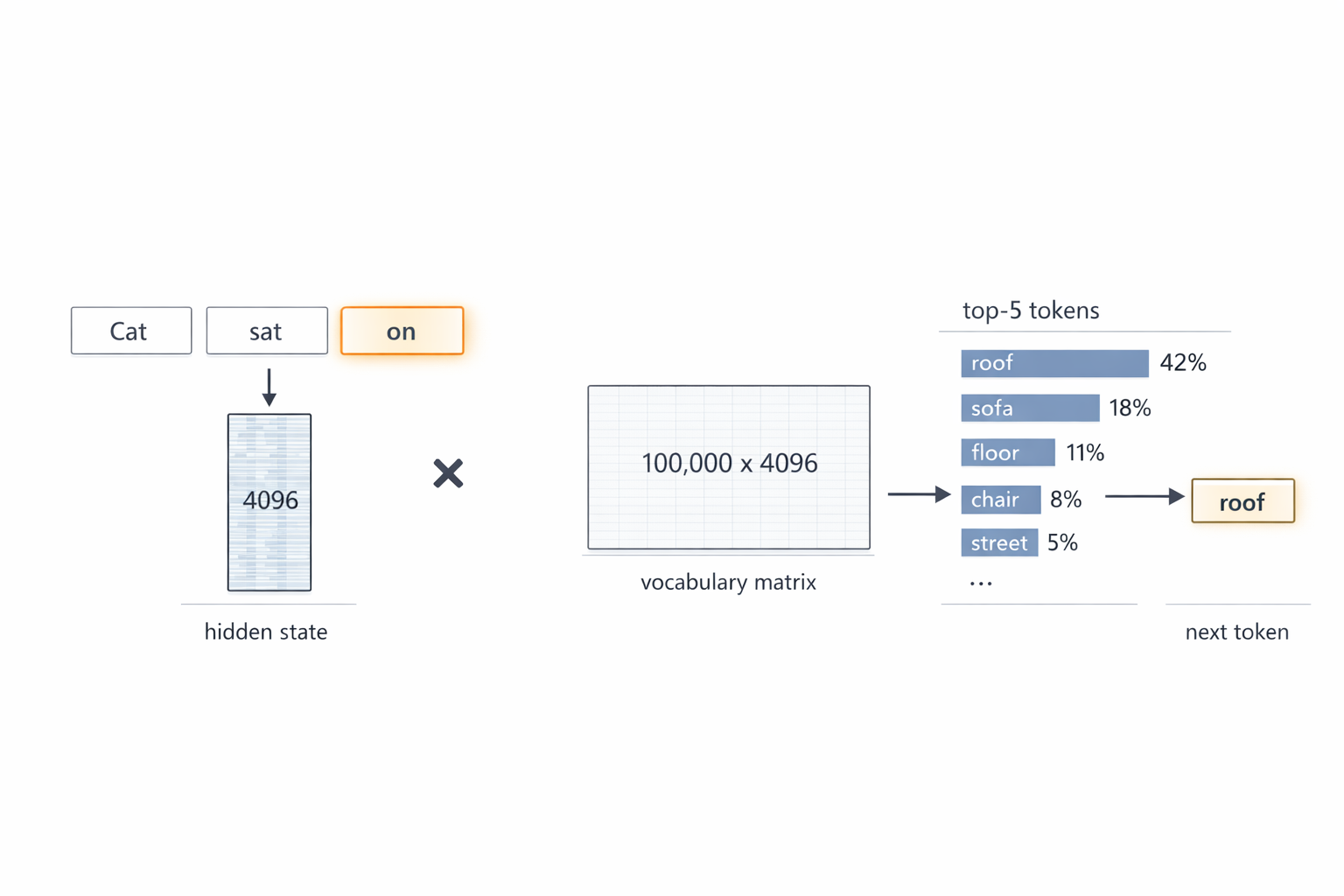
Fig. 3. Input text “The cat sat on” is split into 3 tokens, the last (“on”) highlighted. Its hidden state vector (4096 numbers) is multiplied by the vocabulary matrix (100,000 × 4096) → 100,000 logits → top-5 candidates: roof 42%, sofa 18%, floor 11%, chair 8%, street 5% → next token: “roof”.
3. FFN: The Transformer’s “Knowledge Memory”
Where FFN Lives in the Transformer
FFN (Feed-Forward Network) is part of every transformer layer. Each layer does two things in sequence:
- Attention (words communicate with each other)
- FFN (each word is processed individually)
These two blocks always come as a pair, connected by residual connections (the result is added to the input, not replacing it).
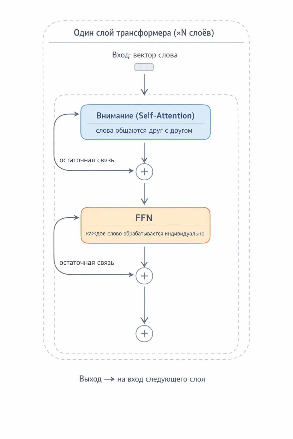
Fig. 4. One transformer layer: Attention block (collective operation — words exchange information), then FFN (individual operation — each word consults the “knowledge library”). Residual connections preserve the original information.
Many such alternating layer pairs stack up — over a hundred in modern models. Without FFN, the transformer is a meeting where no one ever gets to work.
FFN Structure: A Two-Layer Neural Network
FFN is a simple neural network: just two fully connected layers with an activation function between them. No convolutions, no recurrence, no attention — the same perceptron Yann LeCun described back in the 1960s.
The entire FFN mechanic fits in three steps: expand → filter → compress.
The word vector (4096 numbers) enters. The first matrix W₁ expands it fourfold — to 16,384 numbers. This is the working space: the wider it is, the more different “questions” the model can ask at once. The ReLU activation (simple rule — if negative, replace with zero; if positive, keep as-is) cuts out all inactive neurons — of the 16,384, only 2–5% fire on any given word. The second matrix W₂ compresses the active neurons’ answers back to 4096 numbers — the same format used everywhere else in the transformer.
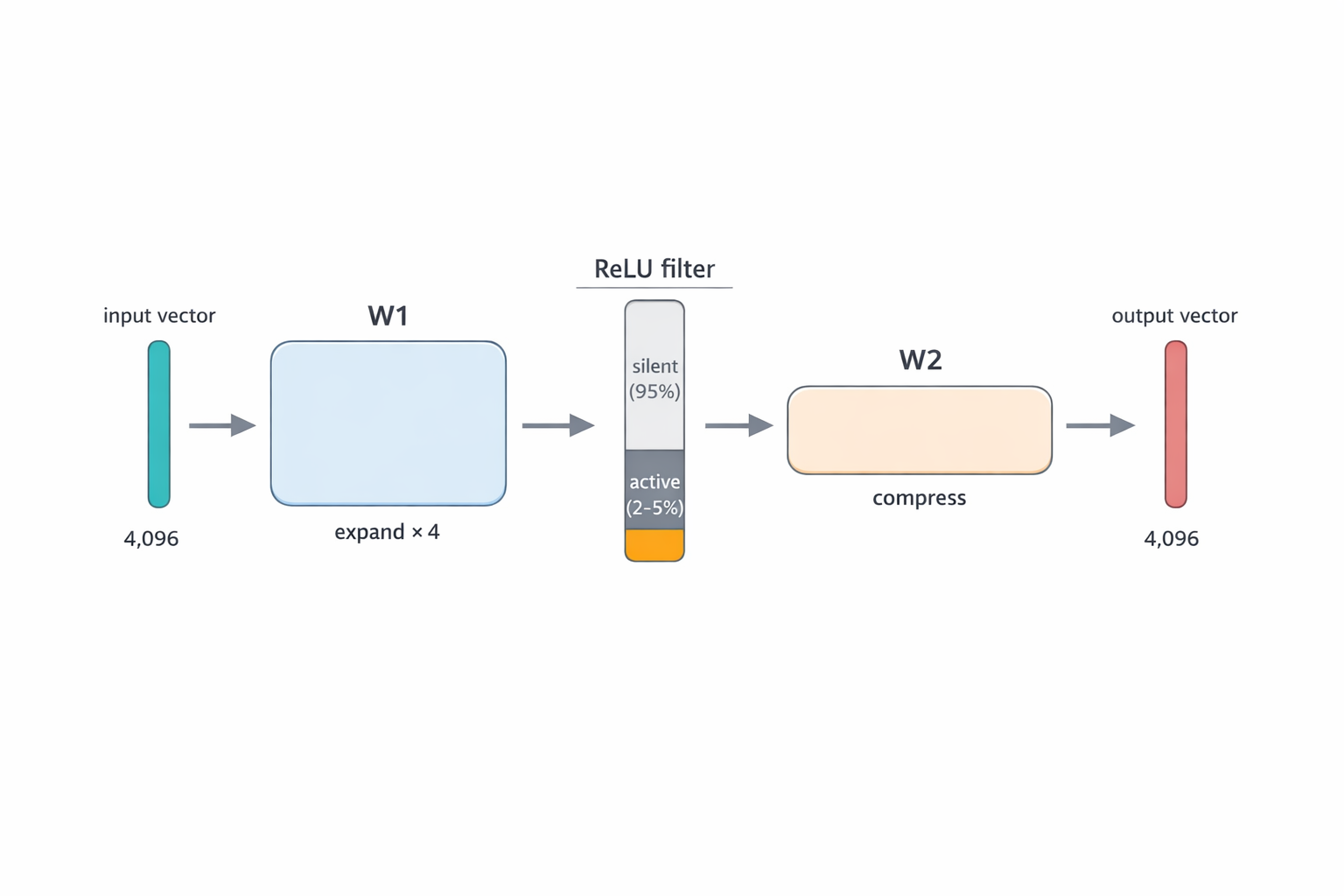
Fig. 5. FFN internals: input layer (4096) → W₁ expands 4× → hidden layer (16,384 neurons, ReLU deactivates inactive ones) → W₂ compresses back → output layer (4096).
What Is Matrix Multiplication (and Why Does It Matter Here)
Before breaking down the three FFN steps, let’s clarify matrix multiplication. No panic.
A vector is simply a list of numbers. A word’s vector in a transformer is 4096 numbers, each encoding some aspect of meaning. Let’s simplify to 4 numbers for the example:
word vector “Minsk” = [0.8, 0.1, 0.6, 0.3]
What do these numbers mean? Roughly: 0.8 — “related to geography”, 0.1 — “related to food”, 0.6 — “a national capital”, 0.3 — “abstract concept”. (In reality the model decides what each number means, but that’s the idea.)
A row of matrix W₁ is one neuron-detector. It too is a list of 4 numbers — the pattern this neuron looks for:
neuron “beautiful capital” = [0.9, 0.0, 0.7, 0.0]
This neuron is “charged” for geography (0.9) and capital-ness (0.7), while food and abstractions leave it indifferent (0.0).
The dot product is a check: how closely does the word vector match the neuron’s pattern? We multiply each pair of numbers and sum:
0.8 × 0.9 + 0.1 × 0.0 + 0.6 × 0.7 + 0.3 × 0.0 = 0.72 + 0 + 0.42 + 0 = 1.14
Result 1.14 — high. The “beautiful capital” neuron fires strongly on the word “Minsk”. Indeed it is!
Now a different neuron — “motion verb”:
neuron “motion verb” = [0.0, 0.0, 0.1, 0.9]
Dot product with “Minsk”:
0.8 × 0.0 + 0.1 × 0.0 + 0.6 × 0.1 + 0.3 × 0.9 = 0 + 0 + 0.06 + 0.27 = 0.33
Result 0.33 — weak. The “motion verb” neuron barely reacts to “Minsk”. Makes sense — Minsk isn’t a verb.
That’s matrix multiplication. W₁ is a stack of 16,384 such neuron-rows. Each row is its own pattern. Multiplying a vector by the matrix simultaneously checks 16,384 patterns in one step. The output: 16,384 numbers, each saying: “how much does the input resemble my pattern”.
Key intuition: matrix multiplication is not abstract math. It’s a massive parallel pattern search. W₁ contains 16,384 “questions”, and every question is simultaneously checked against the input vector.
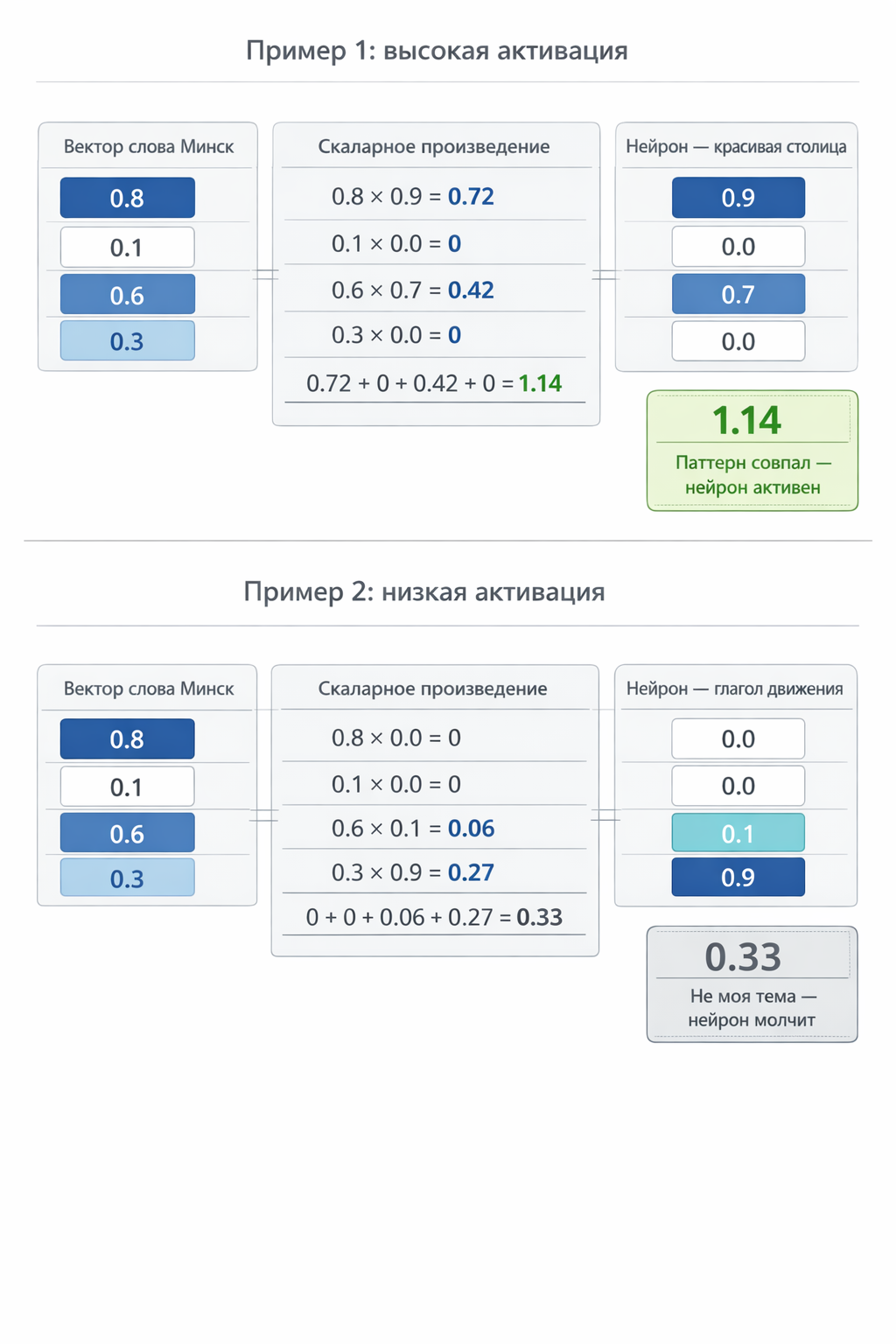
Fig. 6. Dot product — the basis of matrix multiplication. A row of W₁ (neuron pattern) is element-wise multiplied with the word vector, results are summed. High result = “pattern matched”, low = “not my topic”.
Neuron
Let’s also unpack what a neuron actually is. Above we said “a row of matrix W₁ is one neuron-detector”. More precisely, a neuron is a function containing that vector, a bias, and an activation function. But what is a neuron in terms of meaning — not as a simple data structure, but from a phenomenological perspective of the model’s cognition?
I’d define it as an “atom of meaning”. Not in the human sense (like a word in a dictionary), but in a specific, “machine” sense. Let’s break it into levels to try to understand its semantic essence:
A neuron is an elementary unit of abstraction. It is the model’s way of “extracting” one specific facet of reality from a sea of data and naming it (as an activation). As Aristotle said, “true being is activity.” A neuron does not “exist” — it “happens” in the moment of activation. But here’s the problem: neurons are often polysemous. One and the same neuron can react both to “proper nouns” and to “words after a comma.” So its “meaning” is not a clear definition, but a cluster of correlations. As Sheckley put it — “For an illusory entity — an illusory coin” ©. A neuron operates not with the objective world, but with its shadows in vector space. It does not reflect reality directly — it creates a statistical imprint of it.
A neuron is a filter of reality. A question the model asks the world. A human question: “Where am I?” A neuron’s “question”: “How closely does the input vector match my internal tension (weights)?” A neuron’s meaning only emerges in relation. It does not exist on its own. It exists only as a reaction. The neuron’s essence is not an object but an event. It is an act of recognition. Not a semantic entity in a vacuum. It is a coordinate in a multidimensional space of meanings.
A neuron is an elementary act of distinction. It is the minimum unit that says: “This is slightly more like that than like this.” Its weights are not “knowledge” — they are the crystallized experience of testing this hypothesis on millions of examples. When a neuron activates, it does not “recall a fact” — it says: “My hypothesis has found confirmation again.” But without an incoming signal, this mechanism is dead. Recalling Sheckley — “There were no differences, for there was no one to ask about them.” Without the question (input data), a neuron is merely an empty form. Meaning is born only at the junction of question and answer.
How Data Flows: Expand → Filter → Compress
Now that matrix multiplication means “pattern checking”, the three FFN steps become clear:
Step 1 — Expansion (W₁). Word vector (4096 numbers) multiplied by W₁ (16,384 rows × 4096 columns). Each row is a detector neuron with its own pattern. Result: 16,384 numbers, each showing one neuron’s reaction strength. It’s like simultaneously asking 16,384 questions: “Are you a capital?”, “Are you a verb?”, “Are you about food?"…
Why expand from 4096 to 16,384? Because 4096 questions aren’t enough to store all the model’s knowledge. With only 4096 neurons, one neuron has to cover multiple topics. With 16,384 — each topic gets its own dedicated neuron. More detectors = finer specialization.
Step 2 — Filtering (ReLU). After W₁ multiplication we have 16,384 numbers. Some are large positives (the neuron “recognized” its thing), some near zero or negative (the neuron “shrugged”). ReLU does one simple thing: max(0, z) — everything negative becomes zero.
Why this way? Because we need a clear boundary between “neuron active” and “neuron silent”. A weak signal is noise, not knowledge. ReLU says: either you’re confident — or be quiet.
Semantically: a word vector is coordinates in semantic space. Words with similar meaning have similar vectors — they “point” in the same direction. A neuron also stores a pattern-vector. The dot product is the angle between two vectors: if the word and neuron “look” the same direction, the product is large and positive → ReLU passes it. If the neuron is tuned to a completely different topic — product is zero or negative → ReLU zeros it out.
Result: of 16,384 neurons, only 2–5% activate — those whose “specialty” is semantically close to the current word. For “Minsk” in a capital context, geography and politics neurons fire; food, programming, and sports neurons get zero.
Step 3 — Compression (W₂). Now we pack the active neurons’ answers back into the working format of 4096 numbers. W₂ (4096 rows × 16,384 columns) does the reverse: each column of W₂ is a “recipe” describing how an active neuron changes the output vector. Active neurons contribute; silent ones contribute zero.
Why compress back? Because everything else in the model (attention, next layer, final prediction) works with 4096-dimensional vectors. 16,384 is temporary workspace — like spreading folders across your desk. When done, you pack them back into your briefcase (4096) and carry it to the next floor (next layer).
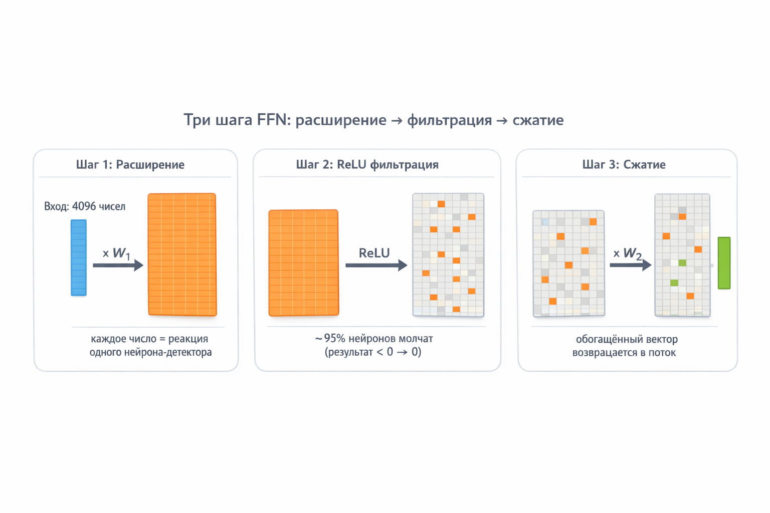
Fig. 7. Step-by-step FFN pass: word vector (4096) → W₁ expands to 16,384 detector neurons → ReLU deactivates irrelevant ones (95% go silent) → W₂ compresses active answers back to 4096.
Example: The Word “Minsk” Through One Layer
Phrase: “Minsk is the capital of Belarus”.
Step 1 — Attention. The word “Minsk” queries all other words and finds “capital” (weight 0.45) and “Belarus” (0.30) most relevant. “Minsk”’s vector is enriched with context — it now “knows” it’s about a capital.
Step 2 — FFN. The enriched vector enters FFN. Of 16,384 neurons, those whose patterns matched activate:
- Neuron “beautiful capitals” → adds: “→ Belarus, wide boulevards”
- Neuron “Slavic languages” → adds: “→ Russian”
- Neuron “postwar architecture” → adds: “→ Independence Avenue”
- Neurons “cuisine”, “programming”, “verb tenses” → silent
Output: “Minsk”’s vector now carries not just the attention context but knowledge: capital of Belarus, Eastern Europe, Russian language.
Key point: FFN works only with the word “Minsk” — it doesn’t look at “capital” or “Belarus”. The context was already received during the attention step. FFN only retrieves knowledge from its own memory.
FFN Across Layers: From Grammar to Facts
FFN does different work at each layer:
Lower layers (1–8) — basic language processing. Neurons react to grammatical patterns: parts of speech, gender, tense, case. The word “bank” in lower layers is simply “noun, masculine, potentially ambiguous” — with no understanding whether it’s financial or riverbank.
Middle layers (9–20) — semantics and disambiguation. If “bank” is near “credit” and “interest” → finance neurons activate. If near “river” and “shore” → geography neurons. The same word gets different “additions” depending on context.
Upper layers (21–32+) — facts and reasoning. Neurons store concrete knowledge: “Minsk → Belarus”, “Berlin → Germany”. Abstract logic lives here too: style, tone, argument structure.
Phrase: “She ran down the dark street because someone was following her”
| Layer 3 (lower) | Layer 25 (upper) | |
|---|---|---|
| “ran” | verb, past tense, feminine, motion | fear, danger, escape, pursuit |
| “dark” | adjective, prepositional, feminine | danger, night |
| “following” | verb, past tense, masculine, motion | pursuit, threat |
Lower layer — the “secretary”: records grammar. Upper layer — the “analyst”: draws conclusions.
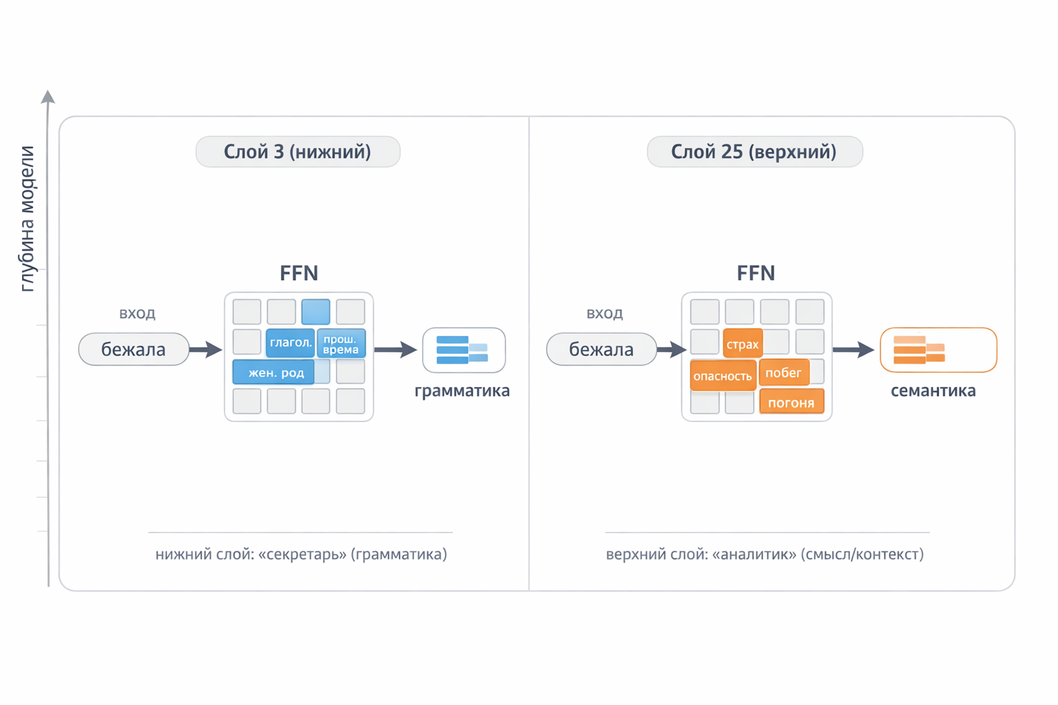
Fig. 8. Lower layers extract grammatical features, upper layers extract semantic ones. The same word, completely different processing.
How FFN Learns: The Story of One Neuron
How does a neuron become a “specialist”? Let’s walk through Neuron #3847, learning to recognize beautiful capitals.
Step 1 — before training. Random weights. The model is shown “Minsk is the capital of ___”, and answers wrong: “Poland”. Neuron #3847 activates weakly and doesn’t help.
Step 2 — error correction. The right answer is “Belarus”. Backpropagation computes: if the neuron reacted more strongly to the pattern “Minsk + capital”, the error would have been smaller. Weights are slightly adjusted.
Step 3 — thousands of examples. The model encounters “Minsk — capital of Belarus”, “Moscow — capital of Russia”, “Skopje — capital of Macedonia” — the neuron strengthens its reaction to the “[city] + capital” pattern. Encounters “Minsk is famous for potato pancakes” — different context, neuron learns to stay silent without the word “capital”.
Step 4 — specialization. After billions of examples the neuron is now a detector: fires strongly on “[city] + capital”, silent in other contexts. Its output weights (W₂) are tuned so that when it activates, it “hints” at the right country.
This happens simultaneously across 16,384 neurons in each of 120 layers. Nobody programmed a “capitals neuron” — specialization emerges from training itself.
Why hallucinations happen? The neuron learned a pattern, not a fact table. Feed it “Wakanda is the capital of ___”, the neuron activates (pattern matched), and the model “confidently” names some country — even though Wakanda doesn’t exist.
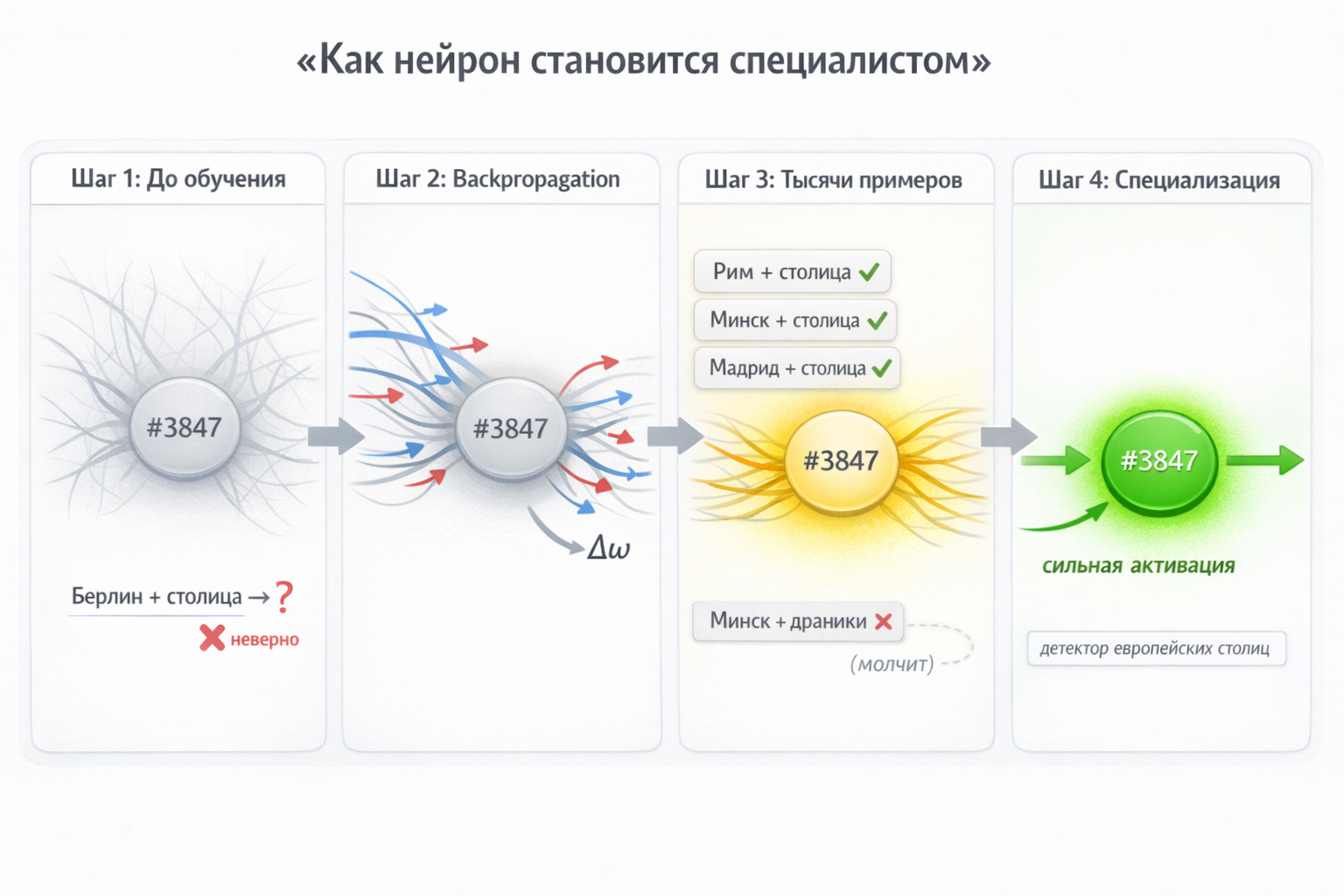
Fig. 9. Four training stages: random weights → backpropagation corrects the error → after thousands of examples the neuron specializes → becomes a “capitals detector”.
4. Hidden States: A Vector’s Journey
What Is a Hidden State
As a token passes through the transformer, its vector continuously transforms at each layer. These intermediate vectors are called hidden states.
- Layer 0 (embedding): the vector holds only the basic word meaning — “cat” = rough representation of cats.
- Layer 4: the vector already “knows” it’s a specific cat from context — “the cat that was on the roof”.
- Layer 32: the vector carries deep understanding — the word’s role in the sentence, connections to other words, emotional tone.
Residual Connections: Memento
An important mechanism — residual connections. After each block (attention, FFN) the result is added to the input, not replacing it:
output = input + block_result
This means the original information is never fully lost — each layer only adds new “meaning layers” on top of the old. Without this mechanism, deep networks couldn’t be trained — information would fade passing through dozens of layers.
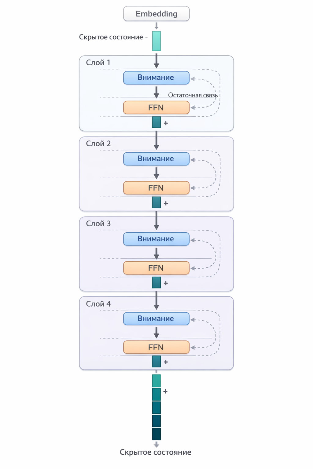
Fig. 10. Vector path through transformer layers with residual connections
5. KV Cache: Speeding Up Text Generation
How KV Cache Forms
Back to the attention mechanism. Each token at each transformer layer produces three vectors:
- Query (Q) — “what is this token looking for?”
- Key (K) — “what does this token offer?”
- Value (V) — “what does it contribute when selected?”
More on Q, K, V — in the previous article.
During text generation the model works step by step: first token, then second, and so on. To generate each new token, attention must compare its Query against all previous Keys and collect Values — essentially re-reading all previously written text. Without optimization: recalculate K and V for every token at every step.
The solution is simple: compute K and V once — then save them. This is the KV cache. Each time a token passes through a layer, its Key and Value are written to cache. When generating the next token, only the new token’s Query needs to be computed; all previous keys and values are pulled from cache directly.
Two processing phases:
- Prefill — user sends prompt. Model processes all tokens in parallel, simultaneously computing and storing K and V in cache for each layer.
- Decode — generation one token at a time. Each new token adds its K, V pair to cache and uses all previous ones for attention computation.
The Price of KV Cache — Memory
KV cache lives in GPU memory and grows with each token. To appreciate the scale: in a model like LLaMA-3 70B with 80 layers, one token produces 80 pairs of K and V vectors with 8192 numbers each — roughly 10 MB per token (in float16). With a 128,000-token context, the cache takes over 100 GB — more than the model itself. This is why context window length is limited not by math, but by GPU memory.
Prefix Caching: “I Already Computed That”
A typical production scenario: thousands of requests to one model. Most start the same way: the same system prompt (“You are a legal assistant, respond formally…”), or the same knowledge base loaded into context. Why recompute K and V for those tokens every time?
So we cache KV not just within one request, but across requests. This is how Automatic Prefix Caching in vLLM works — one of the most popular LLM serving engines.
The hashing mechanism works as follows. The KV cache is sliced into fixed-size blocks — say, 16 tokens each. Each block is hashed by two components: the block’s own tokens and the parent block’s hash (i.e., all preceding text). This creates a hash chain: block 2 depends on block 1, which depends on block 0.
When a new request arrives, vLLM hashes all prompt blocks and looks for matches in the cache table. If the first 12 of 15 blocks are found — they’re taken from cache, prefill only runs for the last 3. A cache hit means: no need to pass those tokens through all 80 model layers — the computation is skipped entirely.
Blocks not recently used are evicted by LRU (Least Recently Used). Only complete blocks are cached — the incomplete last block isn’t hashed until it fills.
Result: with repeating prefixes, response time drops dramatically and the GPU only works on what it hasn’t computed yet.
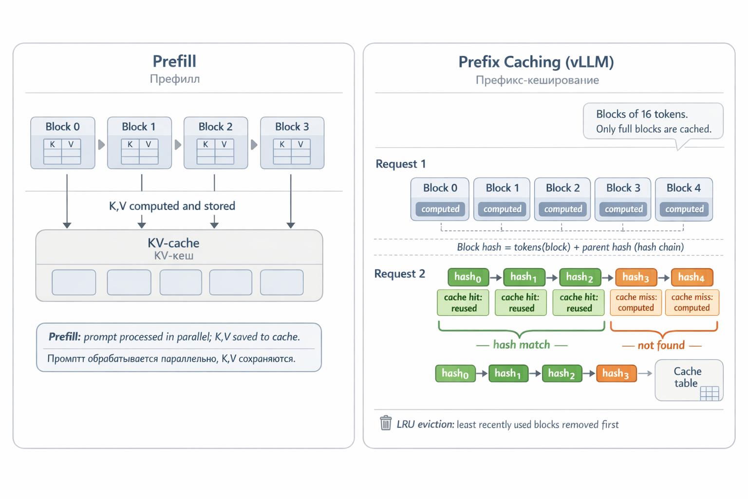
Fig. 11. KV cache: prefill computes K,V for each token. With prefix caching, a new request with the same start finds the first blocks in cache by hash — and skips their computation.
6. How It All Fits Together
Let’s sum up and look at the full picture — from text input to answer generation:
Tokenization — text is split into tokens, each gets a numerical vector (embedding) + positional information.
Layer pass — each token’s vector passes through N layers, each of which:
- Attention: tokens exchange information (Query-Key-Value).
- FFN: each token is enriched with knowledge from the model’s “memory”.
- Residual connections: original information is preserved.
Prediction — the last token’s vector passes through the final linear layer → a probability distribution over the entire vocabulary → the next word is selected.
KV cache — during text generation, keys and values are saved to avoid recomputing everything for each new word.
Repeat — steps 2–4 repeat for each new token until the model has generated the full response.
So It Goes (c) Kurt Vonnegut, “Slaughterhouse-Five”
The core idea: let every word interact freely with every other word. Attention determines what matters; FFN layers enrich each word with knowledge; residual connections preserve information through dozens of layers; and KV cache makes text generation practically feasible.