Dissecting the Transformer. Part 1

In this article the author attempts to make sense of the transformer architecture — everyone has heard of it, everyone “knows” it, yet hardly anyone truly understands it. So the goal here is to explain things at a conceptual level, without arcane mathematical formulas and unreadable definitions. Let’s admit that explaining theory in simple, clear words is a true art, accessible to few of the Landau-and-Lifshitz caliber — but in our age of decadence and postmodernism we shall try as best we can. And yes, the author does not guarantee 100% accuracy of what follows — only his own understanding of it.

So — let’s try to understand what happens to a prompt on its journey from the tokenizer to the triumphant generation of a new token, with stops along the way.

First, let’s look at the overall picture — how the prompt passes through the tokenizer, turns into tokens and their IDs, gets vectors from the embedding matrix, and finally arrives at the input of the first layer. We’ll try to understand what happens at each step and grasp the meaning of it all.

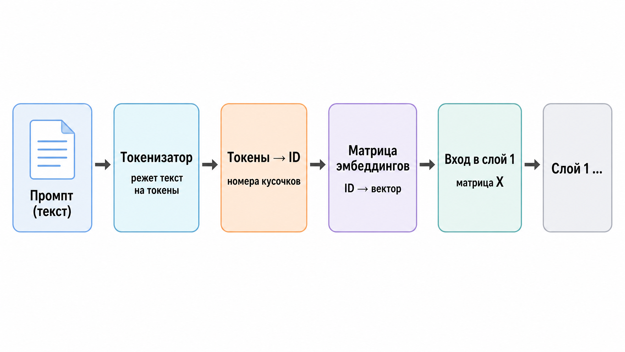
Fig. 1. The prompt’s journey from a bird’s-eye view: details to follow.

Part 1. The Front Gate: the Tokenizer in Detail

It will surprise no one that the model doesn’t work with words — it works with numbers from a fixed vocabulary. So the question is: how do we translate the words of a prompt into numbers? Especially for languages with lots of word forms (inflections, plurals, verb conjugations), and considering that any language keeps evolving, growing new terms and loanwords. What about typos, emojis and the like? So we don’t try to build a fixed dictionary listing every possible word form in advance — we take a different route, the BPE algorithm (Byte-Pair Encoding). During training we use a so-called “greedy” vocabulary-building technique that analyzes the most frequently co-occurring pairs of symbols. This is best explained with an example. Imagine we’re training a tokenizer on a tiny corpus containing the words “low”, “lower”, “lowest”, “below”. We start with an alphabet of individual characters:

l o w e r   b e l o w   l o w e s t ...

The algorithm counts which pair of adjacent symbols occurs most often and glues it into a single new token. Say the most frequent neighbors are l and o → we create the token lo. We rewrite the corpus:

lo w e r   b e lo w   lo w e s t ...

Then we look for the most frequent pair again. Now it’s, say, lo + w → the token low. And so on — thousands upon thousands of merges, until the vocabulary grows to the target size. Every merge is recorded in a merge table — an ordered list of “glue this to that”.

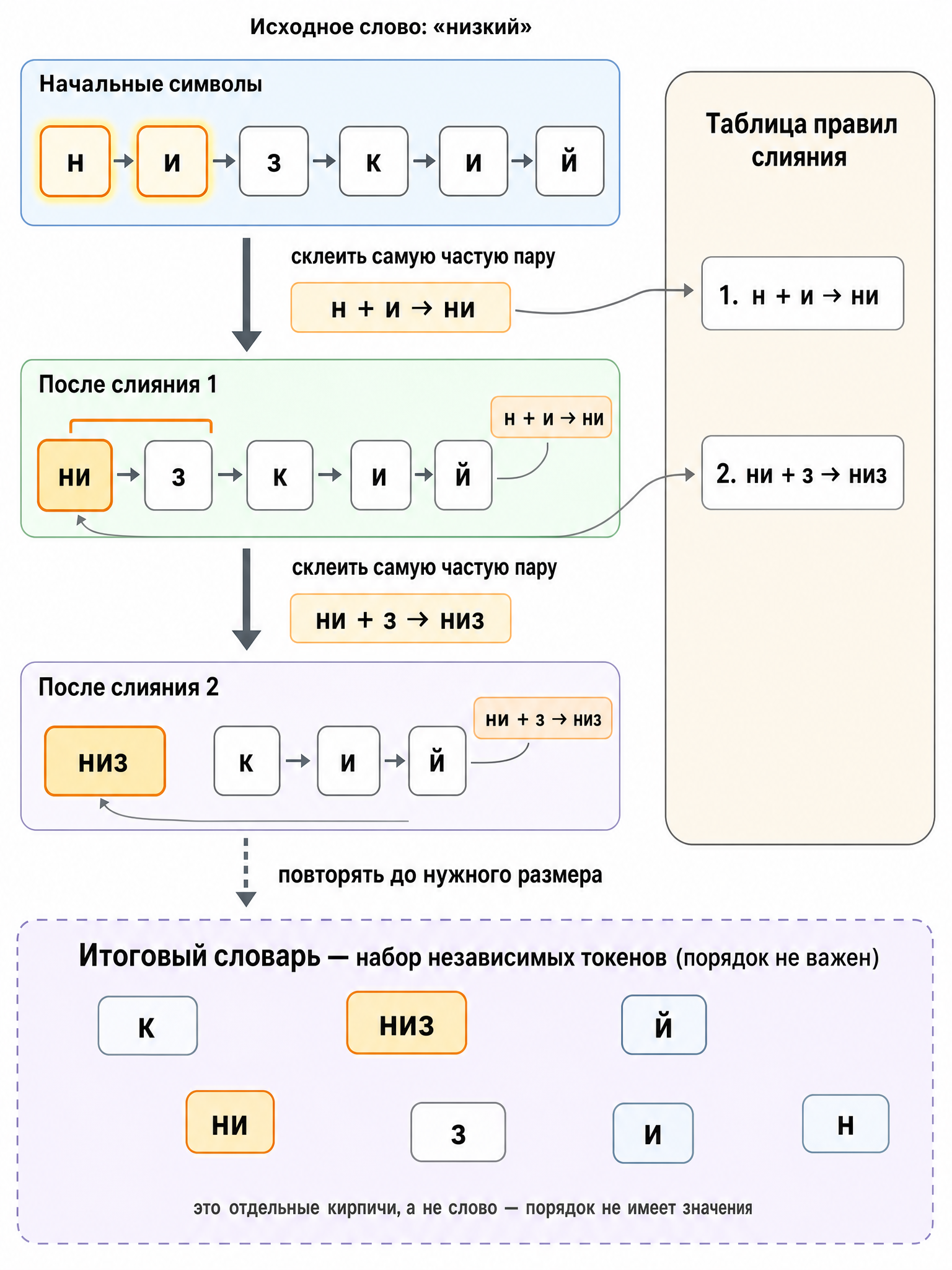
Fig. 2. BPE building a vocabulary: at each step the most frequent pair of adjacent symbols is merged, and the rule is recorded in the merge table.

What we get at the end of tokenizer training — two artifacts:

• The vocabulary itself, i.e. a mapping token-string → integer ID. For example “▁lowest” → 5567, “low” → 4021, “lowe” → 903, “est” → 231, “t” → 68.

• The merge table: the set of “glue this to that” rules; this is precisely what assembles tokens from individual characters when parsing new text.

The important thing about this approach is that there are no unknown words at all — since every individual character is already in the vocabulary, we’re merely trying, using the merge table, to assemble something out of them. And if the prompt contains a meaningless jumble of characters, no merge rule will apply and the jumble stays scattered into individual characters. So if a cat walks across your keyboard and produces xqzrwvk, the tokenizer will first slice the sequence into individual letters, find no familiar pairs in the merge table — and leave everything as is: 7 separate tokens. There’s no meaning in them, of course, but the point is the model could still encode them, which means any text whatsoever gets through.

By the way, remember how older models couldn’t count letters in words (how many r’s in “strawberry”?). That’s precisely a consequence of the tokenizer: to the model, that word is a single token with some ID — the model doesn’t know what letters are inside. Later this got solved — either through “reasoning” (the model spells the word out into individual character tokens) or through tools (generating code to count the letters).

Another curious bit: spaces. I too used to think spaces were separate tokens — but it turns out that in many tokenizers a space is not a separate token but part of another token. That is, cat (with a leading space) and cat are two different tokens. More precisely, the space does also exist as a standalone token — for instance, with cat the first two spaces end up as two separate tokens, and the third token is cat (with one space). Why such complications? Well:

1. Token economy: there are roughly as many spaces in text as there are words, so the token count would double. This way the space rides along inside the word for free — fewer resulting tokens, hence less computation downstream.
2. A word-boundary marker — a hint to the model that “a new word starts here”. It disambiguates two cases of the same letters:
   • cat — the word “cat” standing on its own.
   • cat (no space) — the same letters as a continuation of another word (say, inside “concatenate” or a compound token).

So gluing the space onto the word is the cheapest way to mark word boundaries without paying a separate token for every space.

Now an Example

Let’s trace the fate of a simple prompt: The cat was sitting on the roof. The prompt arrives at the tokenizer, which slices it, say, like this:

"The"      → [88123]
" cat"     → [4517]
" was"     → [902]
" sitting" → [312, 7745]     # " sitt" + "ing" — the word broke into two pieces
" on"      → [15044]
" the"     → [1996]
" roof"    → [8873]

Total: [88123, 4517, 902, 312, 7745, 15044, 1996, 8873] — 8 tokens out of 7 “human” words. And note — the spaces rode along inside the tokens, and one word split into two chunks. These eight numbers are what the model will work with from here on.

The Embedding Matrix

“Embedding” is one of those terms that resists a plain-language translation; the closest rendering in our context is probably “matrix of vector representations”. The size of this table is the model’s vocabulary — every token it knows. And the columns are the coordinates of a given token in “semantic space”. The number of columns is set when the model is designed — 4096, for instance. Each one is some dimension of semantic space — say “size”, “animacy”, “sentience”, “past tense” and so on.

So, for example, suppose embedding(" cat") = E[4517] → a vector of 4096 numbers. Accordingly, tokens close in meaning will sit near each other in this multi-dimensional semantic space. We can’t picture that many dimensions — but think of our Milky Way galaxy by analogy: as if the stars were tokens, and those close in meaning sit near one another. “Dog” will be near “cat” and “ferret”, a bit further out “blue whale”, and “tractor” somewhere far away. But axis names like “size” or “animacy” are merely a convenient illustration. In reality an individual coordinate usually has no human-readable meaning: one feature is smeared across many dimensions, and one dimension encodes a blend of features. And this basis wasn’t specified by us in advance — the model derived it itself during training, from the statistics of next-token prediction, choosing whatever decomposition turned out convenient for it.

In other words, what matches our picture of the world is not the meaning of individual dimensions but the geometry of the space as a whole: proximity and relative positions of tokens reflect semantic relationships we recognize — “dog” next to “cat”, and the classic “king − man + woman ≈ queen” works like ordinary arithmetic. Which makes sense: the model learned from human texts. Only the dimensions themselves are inscrutable to us — what got decomposed along which axis is hard to tell. But we don’t need to: meaning lives not in individual columns but in the distances and directions between points.

Onward to the First Layer

So far we’ve dealt with processing a single token — but let’s return to our original prompt The cat was sitting on the roof. We have 8 numbers, and we get 8 vectors as described above (8 × 4096) — that is, a matrix. That matrix is what gets sent into the first transformer layer.

But before shipping it off — one non-obvious point: word order. It might seem like a non-issue — the rows are right there in order: first “The”, then " cat", and so on. The problem is that the model doesn’t read the matrix top to bottom the way we read text — it processes all 8 vectors at once, in a single operation, and the row number plays no part anywhere in those computations.

The fix: since the model only looks inside vectors, the position has to be stuffed inside the vector too — right into those 4096 numbers. The model itself does this (not the tokenizer) — a simple deterministic operation that mixes each vector’s sequence number into it. As a result the model no longer sees “a cat in general” but “a cat standing second in the sequence”.

Older models added a separate “positional vector” PE[i] to the token vector — a distinct set of numbers per position — but we’ll jump straight to the modern method of “baking” position into the vector: RoPE (Rotary Position Embedding). The essence: a token’s position is encoded by rotating its vector. Sounds cryptic so far — don’t panic, we’ll take it apart in detail.

What does it mean to rotate a vector? A token’s vector is, in our example, 4096 numbers — the coordinates of a point in semantic space. Mentally draw a line from zero to that point — you get an arrow; the point and the arrow are the same thing, two views of the same numbers. To rotate the arrow means to slide the point along an arc around zero: its distance from zero stays the same, but its coordinates change. On a plane with two coordinates it looks like this: “cat” was [1, 0] — an arrow pointing right; rotate it 30° — it becomes [0.87, 0.5] — the same arrow, tilted slightly upward. With 4096 numbers it’s exactly the same, just impossible to draw.

On the other hand — we established that coordinates are a location in semantic space. Recall where meaning actually lives: “in the distances and directions between points”. Not in the numbers themselves — individual coordinates are unreadable anyway — but in the distances and directions to other words: a cat is a cat because it sits near “dog” and far from “tractor”. Meaning is not a point’s address; it’s the point’s position relative to other words.

Now watch what the rotation actually does. Every word in the prompt gets rotated by the angle of its position: the first word, say, by 0°, the second by 30°, the third by 60°. So the words are rotated by different amounts — and the angle between any two words has changed. Suppose there was some semantic divergence between the tokens " cat" and " was", say 20° — now it’s 20° plus a 30° extra twist (they’re neighbors, one position apart, hence 30°). And that’s exactly where position got mixed in: the angle between two words now contains two terms — the old semantic angle plus an increment exactly proportional to the distance between the words in the text.

The key point: this increment is not random but strictly known — adjacent words are always twisted 30° relative to each other, words two positions apart by 60°, and so on everywhere, in any text, always the same. The semantic part of the angle hasn’t gone anywhere — it sits inside the sum, and the model, having trained with this rule from birth, extracts it from there: it knows that words at adjacent positions come with an “expected” 30° twist, and anything beyond that is meaning. Roughly speaking, we didn’t erase the old writing — we wrote a second layer on top of it in a different color, and a reader who knows about both colors reads both.

And a cat stays a cat because the increment by itself demands nothing of the word: “cat” at position 0 and “cat” at position 100 are the same vector rotated by different amounts, and when compared to any word standing, say, three steps away, the picture is exactly the same — at the beginning of the text or at the end. The word hasn’t changed — only its “place-in-line stamp” has, and that stamp is constructed so that only the difference between stamps matters, never the stamps themselves.

The vector is rotated by a formula hardwired into the model’s code, inside the attention mechanism (we’ll get there). And it rotates not the original but working copies of the vectors that attention makes for comparing tokens — the source vector lies untouched. It’s important to understand: the rotation isn’t some external interference the model had to get used to. It was switched on during training — every text the model ever learned from passed through the very same rotations, by the very same rule. In other words, the model has never in its life seen words without rotations — everything it knows about how words relate to each other was learned on rotated vectors from the start. We read text left to right and don’t consider that a distortion — it’s just how text is written. Likewise, for the model, a rotated vector is the only notation it has ever known.

To sum up: a vector is an arrow, all arrows rotate by a common rule, meaning lives in relative arrangement and therefore doesn’t suffer, and the angles between positions carry the information about word order. For illustration we’ll keep drawing on a plane with two coordinates. Say the word “cat” has vector [1, 0] — an arrow pointing due right. Then rotation by position looks like this:

position 0:  rotation 0°    →  [1.00, 0.00]   arrow right       →
position 1:  rotation 30°   →  [0.87, 0.50]   slightly up       ↗
position 2:  rotation 60°   →  [0.50, 0.87]   steeper up        ↗
position 3:  rotation 90°   →  [0.00, 1.00]   straight up       ↑

Now look at the illustration below explaining the idea — it has two halves.

The left half is our rotation table drawn as arrows: the same “cat” fanned out, from “position 0” (pointing right) to “position 3” (straight up). The word itself doesn’t change — only the tilt does, and the tilt encodes the position.

The right half is about how the model will read those tilts. Here we have to jump ahead again to the attention mechanism: inside a transformer layer, tokens are constantly compared pairwise — “how relevant are you to me?” — and mathematically this comparison depends only on the angle between two arrows. The tilt of each individual arrow plays no part whatsoever — only the spread of the angle between the pair. The two vectors A and B in the right half are two tokens from our prompt, each rotated by its position’s angle, and the arc between them is the only thing the model will see when comparing them.

It’s starting to add up: the angle between A and B is the difference of their rotations — that is, the difference of their positions times 30°. Let’s check with numbers: tokens at positions 2 and 5 — rotations 60° and 150°, with 150° − 60° = 90° between them. The same two tokens at the end of a long text, at positions 100 and 103 — the rotations are now enormous, 3000° and 3090°, but between them it’s still the same 90°. So however much has been “wound up” onto each token individually, it’s invisible in the comparison; only the angle between the pair is visible, and it depends on a single fact: the tokens stand three steps apart.

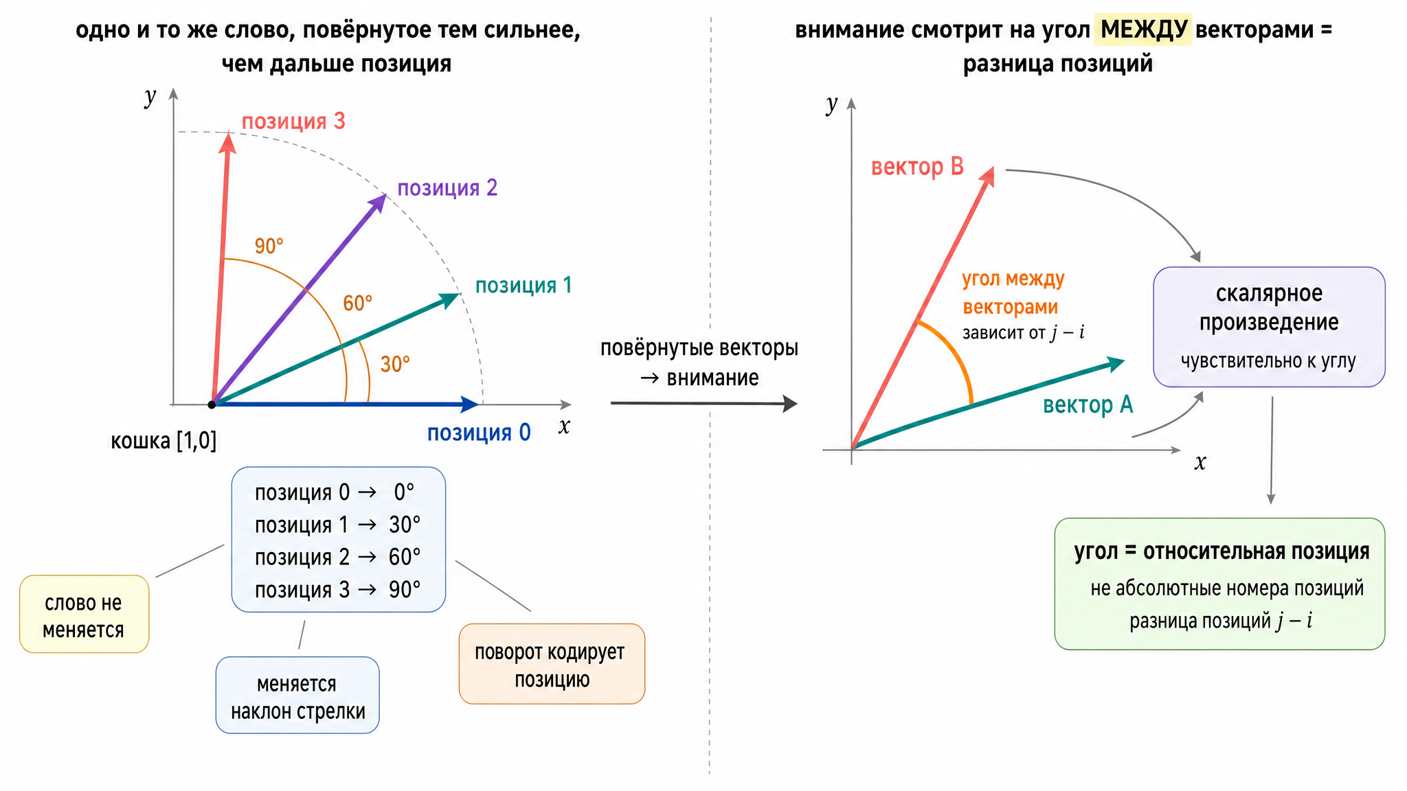
Fig. 3. RoPE. Left: the same word, rotated more the farther its position. Right: attention looks at the angle between vectors, and that angle depends only on the difference of positions.

And here’s the beauty of it. An added positional vector encodes an absolute address: “you are token No. 100000” — and if the model never saw texts of that length during training, the address is gibberish to it, and quality degrades on long texts. Rotation, on the other hand, encodes relative distance: “you two stand three steps apart” — a pattern the model has seen millions of times, at every possible position. Wherever a pair of tokens ends up — at the start of the text or at the hundred-thousandth position — their mutual geometry is identical. That’s why RoPE holds up so well on long contexts and became the de facto standard.

For the purposes of this article it’s enough to understand: by the time it enters attention, each token “knows” its position.

Let’s recap the whole journey from prompt to first layer. There were four transformations: first the tokenizer sliced the text into tokens using its two tables (vocabulary plus merge rules) and produced IDs instead of text. Then, for each ID, a row was pulled from the embedding matrix — a vector of 4096 numbers, the token’s coordinates in semantic space. The rows were stacked one under another — yielding an N × 4096 matrix, in our example 8 × 4096. And finally, positional information was mixed into the vectors — by rotations, as we just covered. That is what rolls into the first layer: no longer text, but not yet any kind of “understanding” — just numbers recording what each token means and where it stands.

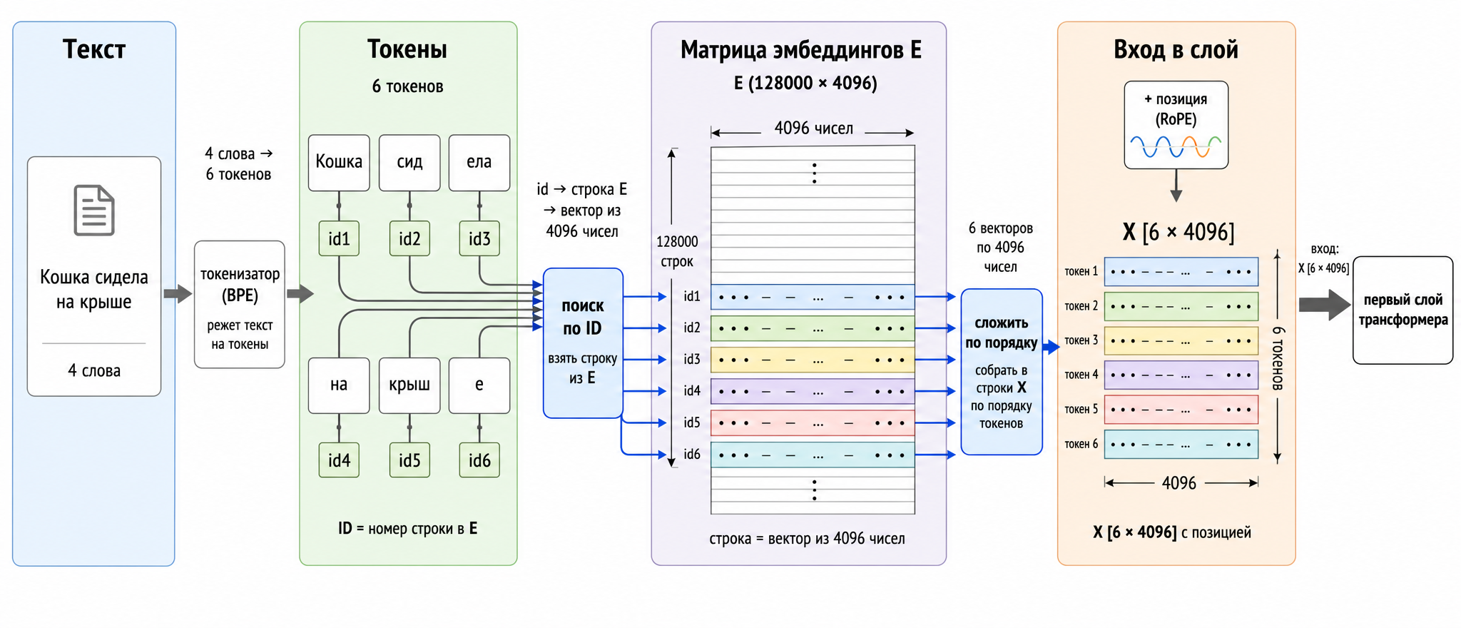
Fig. 4. The full path through the front gate: text → tokens (BPE) → integer IDs → rows of the embedding matrix → matrix X [N × 4096] + position.

Dissecting a Layer

To start with: a transformer layer consists of “attention” and an FFN (Feed-Forward Network — an ordinary fully connected neural net that processes each token independently).

Let’s begin with attention — why does it exist, and what problem does it solve? Recall what rolled into the first layer: a matrix where each token has its vector from the embedding matrix. But these are dictionary meanings — “cat in general”, “sitting in general”, “roof in general”. Each vector describes its token in isolation from the rest, like an entry in a dictionary. What we need is to capture the meaning of the whole sentence. Who was sitting, where — all that information is in the sentence, but how do we tie these tokens together into a semantic picture of “a cat on the roof”?

But wait — didn’t we say above that " sitting" was sliced by the tokenizer into " sitt" and “ing”? So we sort of have a fragment problem. True — but let’s agree on why we’ll keep talking about “sitting” as a single token from here on. First, one of the earliest jobs attention does in the lowest layers is precisely gluing such fragments back together: the token “ing” first of all finds its neighbor " sitt" (a query along the lines of “I’m a suffix looking for my stem” meets a key saying “and I’m a stem missing its ending”) and absorbs it — after a couple of layers the vector at the “ing” position effectively carries the meaning of the whole word “sitting”. Second, don’t confuse this token with other uses of the same letters: the fragment ing without a leading space occurred in training texts almost exclusively as the tail of verbs, and its dictionary meaning is exactly that. So the gluing is also a function of the model — and from here on we’ll treat “sitting” as one token.

Attention is the mechanism by which tokens exchange this kind of information. In a single pass through a layer, each token “surveys” all tokens to its left, decides which ones matter to it, and mixes their content into its own vector. Mixing in means updating its coordinates — adding something to its vector and obtaining a new vector, shifted in semantic space in the direction dictated by context. Simplified for now: each token gets enriched with the meanings of the tokens before it. So “sitting” absorbed “cat”, and “roof” absorbed “on”, “cat” and “sitting”.

To implement such a mechanism, every token needs to be able to do three things: articulate what it’s missing; be findable when its content is needed by others; and hand over its content when chosen. These three roles are exactly what the three vectors — Q, K and V — are for: what to search with, what to be found by, and what to hand over.

• Query — what the token goes searching with. A vector asking, “respond, all who are relevant to me!” For “sitting”, the query would be something like “seeking a subject: who or what performed the action, third person”.
• Key — what other tokens find this one by. A vector encoding “here are my features”: for “cat”, the key says “I’m a noun, third person, animate.”
• Value — what the token hands over if found. A vector with a detailed inventory of features: for “cat” — its attributes “animal, furry, predator, mammal”.

By comparing one token’s query against the keys of all tokens to its left, attention decides whom to take information from; and what it takes is the values. Why can’t we get by with a single vector and compare tokens directly? Because “relevant” is not the same as “similar”. A direct vector comparison would find other verbs for “sitting” — they’re nearby in semantic space. But it doesn’t need a similar verb; it needs a subject. Which means you must search by one feature, be found by another, and hand over a third. Hence three roles, each with its own representation of the token.

Now, where do these vectors come from? They’re the result of transforming the token with the corresponding matrices W_Q, W_K, W_V.

These matrices:

• are created during training and are immutable at inference;
• are distinct for every transformer layer;
• reside permanently in VRAM;

They’re needed to pull those three slices — query, key and value — out of the token vector, where its entire dictionary meaning lies in one lump. Each matrix makes its own slice: W_Q the query, W_K the key, W_V the value. And it’s important to understand what kind of “slice” this is. A matrix is just a table of numbers, and recall matrix multiplication: each number of the new vector is a weighted sum of all 4096 numbers of the original, where the weights are numbers from the matrix (each output number has its own column of weights). So the matrix decides which coordinates of the source vector to amplify, which to mute, which to blend — and what makes it into the result. These weights were tuned during training, on billions of sentences: training ran until, from any token, whatever vector it arrived as, W_Q reliably began extracting exactly “what this token lacks”, W_K “what to find it by”, and W_V “what it can hand over”.

And when you hear “the model has such-and-such many parameters” — that means the total count of trainable weights: these three matrices on each layer are only a part; the total also includes the embedding matrix, the matrices of the layer’s second block (the FFN, more on it later — and that, incidentally, is the lion’s share), and the output matrix (which sits at the very end of the model and turns the final vector into a next-token prediction — we’ll get there too).

The matrix dimensions work like this: the number of rows depends on the length of the input vector — in our example that’s 4096 numbers, so 4096 rows (recall matrix multiplication: the vector is multiplied against the matrix column by column — each number of the vector multiplies the corresponding number of the column, the products are summed — and one column collapses into one number of the result; that’s why the vector’s length and the column’s height must match). The number of columns is the length of the output vector — as many columns as there are numbers in the result — and this one is the model designer’s choice: in our example also 4096, but it can be made smaller.

Now let’s return to our prompt The cat was sitting on the roof and trace the whole process on the token “sitting” (as agreed — treating it as a single token). This word is clearly missing context: who was sitting? sitting where?

Step one — our token gets its trio of vectors. The input is the token vector of “sitting” — 4096 numbers, its dictionary meaning: encoding something like “verb, continuous action, the act of sitting, a posture of rest”. Multiplying this vector by the three matrices yields three different vectors — one per role:

• multiply by W_Q — get the query q (4096 numbers). W_Q is trained to extract from the source vector “what this token lacks”. A verb lacks an agent and a place — so q comes out as something like “seeking a noun-subject, seeking an indicator of place, third person”;
• multiply by W_K — get the key k. W_K extracts “by which features others might look for me”: for “sitting” that’s “I’m a verb, I’m an action, I’m a predicate” — exactly how those in need of a verb will search for it;
• multiply by W_V — get the value v. W_V packs “what I’ll hand over if chosen” — the actual semantic payload: the act of sitting itself, the continuous aspect, a shade of stillness.

(The quoted features are for illustration: in reality these are all the same unreadable coordinates, but in intent that’s precisely the job the matrices are meant to do.)

Note — all three vectors are pulled from the very same source vector, but they’re three different slices of it: what I need, how to find me, what I’ll hand over. And every one of the tokens in the prompt does the same: for “cat”, q will seek a verb (“what was I doing?”), k will announce “I’m a noun, animate, a subject candidate”, and v will carry the cat’s attributes. At this step tokens still know nothing about each other — each prepares its trio alone, out of itself. Technically all of them are pushed through the matrices at once, in a single multiplication — but that’s pure GPU optimization; in meaning it’s independent “token times matrix” operations.

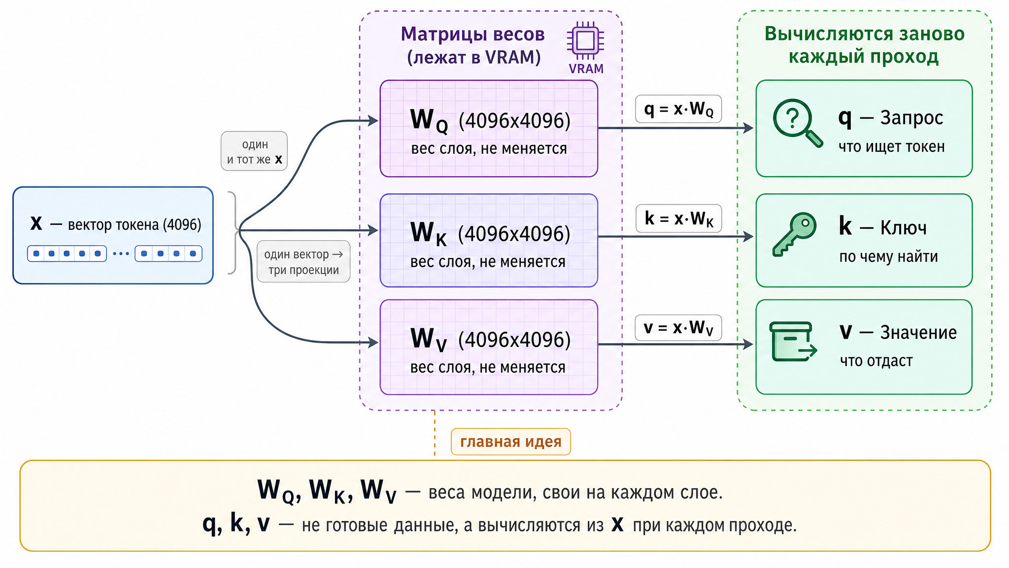
Fig. 5. One token vector, three trained matrices — three roles: query (Q), key (K), value (V).

And to let the matrix roles finally settle in, a simple rule: W_Q and W_K together decide who will look at whom — the structure of connections between tokens. W_V decides what exactly will flow along those connections — the content. The first two draw the attention map; the third prepares the cargo to be carried along that map.

Step two — queries meet keys. Now the tokens start interacting. The query q of the token “sitting” is compared against the key k of every prompt token to its left (including its own) — the comparison is that very dot product, sensitive to the angle between vectors. Looking to the right is forbidden — and that’s not a whim but the essence of a generative model: it learns to predict the next token, and if a token could peek rightward, training would turn into cheating off the answer sheet. So “sitting” sees only “The”, “cat”, “was” and itself, while “roof”, standing at the end, sees everyone. The output — one number per accessible token: how strongly each one’s key “responded” to the query of “sitting”. The query was “seeking a subject” — and the key of “cat” (“I’m a noun, animate, third person”) will produce a large number. The result is an interest profile: who matters to “sitting” and who doesn’t.

Step three — scores turn into percentages. The raw numbers are run through a normalization that turns them into fractions summing to one. “Sitting” doesn’t have much to choose from: roughly 70% on “cat”, 30% on itself. Whereas “roof” has a richer profile: say, 40% on “cat”, 25% on “sitting”, 15% on “on”, the rest on itself. That is the attention distribution: each token has decided how much to look at whom among those it can see.

Step four — collecting the take. Now “sitting” takes the values v from the accessible tokens — not in full, but proportionally to the percentages: 70% of “cat”’s value, 30% of its own. All of it is summed into a single vector — an increment blending the content of the relevant tokens in the right proportions. And this increment is added to the original vector of “sitting” — remember “mixing in means updating coordinates”? This is exactly that: old vector plus increment equals new vector, shifted in semantic space wherever the context dictated. “Sitting” is no longer “sitting in general” but “sitting — and it’s a cat doing the sitting”. As for “sitting where” — that’s no longer its concern: the full picture of “the cat sitting on the roof” will be assembled by tokens further right, who can see the whole sentence.

And every token in the prompt performs this procedure simultaneously — each with its own query, its own interest profile and its own increment. One pass through the layer — and all eight vectors have shifted, each having absorbed its own share.

A fair question here: why enrich all the tokens? After all, when generation time comes, the model will predict the next word from the vector of the last token — that’s the one that must soak up the meaning of the entire sentence. The answer: there are many layers, and each has its own job — its own W_Q, W_K, W_V matrices, trained to extract different things. The lower layers assemble grammar — exactly our example: “sitting, and it’s a cat”. The middle ones compose those linkages into a coherent image of a cat on a roof. The upper ones handle the most abstract: what the sentence is about, its tone, emotional coloring, where it’s all heading. Each level builds from what the previous one prepared — which is why the previous one must enrich all tokens, not just the last: those are its blanks for the next floor up. And so, layer by layer, meaning flows toward the last token — through the vectors of all the others.

Well, the second part of a transformer layer — the FFN — we’ll cover in Part 2 of this article.