On-Prem LLM Deployment: Our Cow, Our Milk
Who’s to blame? What’s to be done? (classic Russian questions)
We’ve been noticing that in our turbulent, multipolar-world-in-the-making era, more and more requests are coming in for on-prem LLM deployments. There are plenty of hidden pitfalls and not much accumulated experience — so let’s try to work through it.
— How’s the project going?
— We’re in the final stage!
— Great, are you wrapping up?
— No, we’re looking for someone to blame!
So here comes a client with a typical wishlist: we want everything inside a closed perimeter. The AI assistant should chat with customers in their language, never leave the corporate network, only answer based on vetted documents, and at the first sign of doubt — hand off to a live operator. Oh, and also: connect all departments, generate management reports, lift conversion to the sky, run all business processes, pass regulatory audits, fit within a fixed budget with a multi-year guarantee. And can we see a demo the day after tomorrow?
And now the fog of questions rolls in:
- Which open LLMs can actually handle all this?
- What hardware do they need?
- How do you handle auto-scaling?
- How much does it cost?
- What if something breaks?
- How do you get acceptable inference for 5,000 users?
- Are you sure the data won’t leave the perimeter?
- If voice input is needed — is that completely different hardware?
- Do open model licenses allow commercial use without restrictions?
- What team is needed to keep this all running?
Let’s dig in
Let’s work through it. The first thing that comes to mind is GPUs. We definitely need some of those…
But that’s just one part of the whole organism — let’s first introduce the concept of an inference node: a single physical server running the model that handles requests to it.
The GPU does the computing. And the question “what matters most in it?” has no single answer: both compute power (teraflops) and VRAM capacity and bandwidth (GB/s) matter. Which one becomes the bottleneck depends on what the model is actually doing at any given moment. And it does two very different things.
The prompt processing phase (prefill). Your entire input text arrives at once, and the GPU processes all tokens simultaneously. The model weights are read from VRAM once — and thousands of tokens are pushed through them immediately. Lots of computation, relatively few memory reads. In this phase the GPU is genuinely busy and hits compute limits.
The generation phase (decode). The response is produced in a fundamentally different way — one token at a time, strictly sequentially, because each next token depends on the previous one. To generate just one token, the GPU must re-read all model weights from VRAM (this is a simplification — in MoE architectures only a subset of weights is read, but the idea holds). The entire model has to be pulled across the memory bus, while the actual computation is trivial (essentially a matrix-vector multiply). The GPU spends most of its time just waiting for data to arrive from memory. In this phase, what matters isn’t teraflops — it’s memory bandwidth.
So the bottom line: decode generates few tokens but takes a long time because each token is a full model read. Prefill is the opposite: it processes thousands of tokens but can finish in fractions of a second.
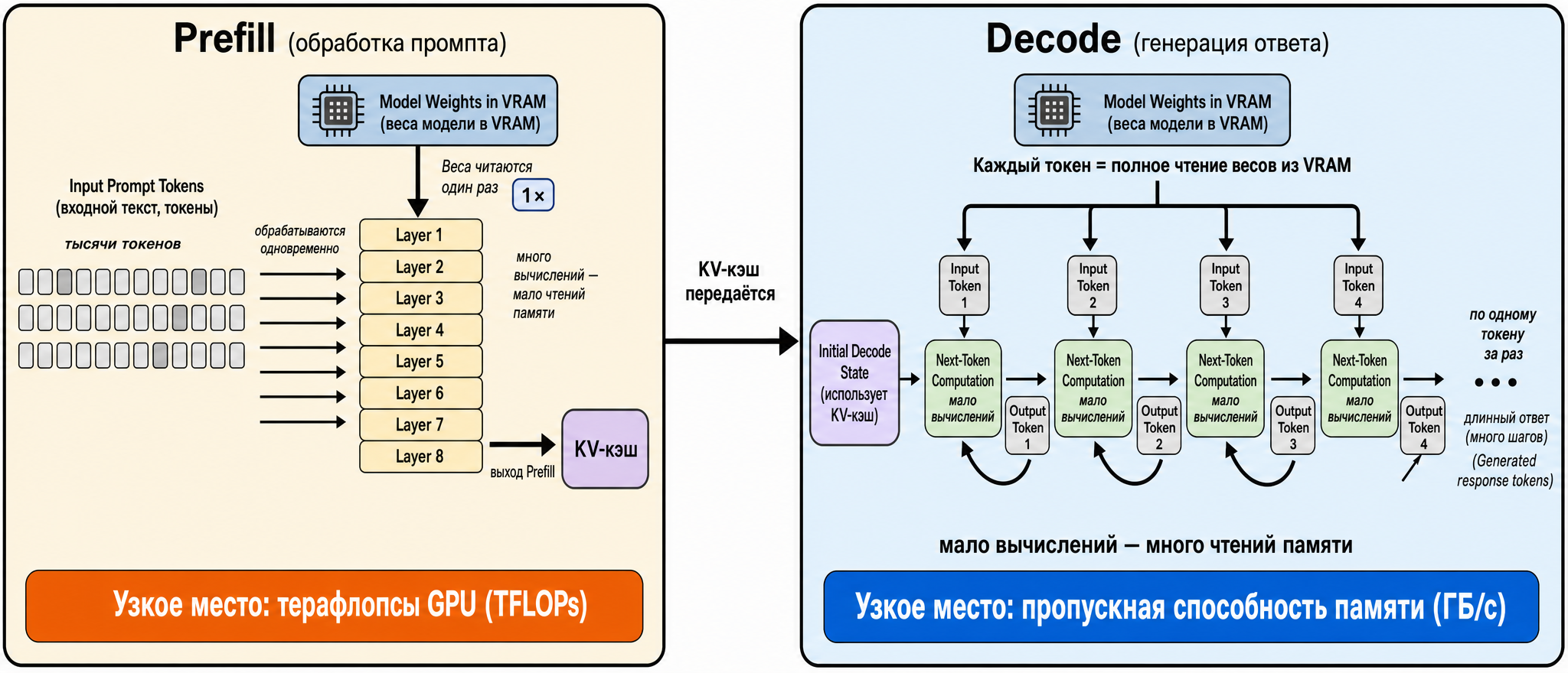
Fig. 1. Two LLM inference phases: prefill is compute-bound, decode is memory-bandwidth-bound
So depending on the workload, either compute or memory matters more:
- Long input, short output — summarization, RAG, codebase analysis. Prefill dominates, and GPU compute becomes the bottleneck.
- Short input, long output — regular chat, text generation, explanations. Decode dominates, and VRAM bandwidth is the limiting factor.
The most interesting case (at least for me) is multi-agent systems — what happens there?
Let’s look at how one agent step works. To decide what to do next, the model re-reads the entire accumulated context every time — the system prompt, conversation history, contents of files it has read, results of previous tool calls. And it produces very little on this step — a tool call, a small patch, a few lines of reasoning. And there are dozens of such steps per task. So every tiny output is paired with an enormous and constantly growing input.
It turns out that an agent does heavy prefill over a large context on nearly every step, with a lightweight decode. The longer the session runs, the more the context balloons — and the more compute-heavy each step becomes. This is why agentic code generation is closer to “long input” workloads — and it hits GPU compute limits.
But — as always, there are nuances. Because there’s a thing called context caching (KV-cache, also known as prompt caching) — more details on that in the transformers post.
The model runs input tokens through all its layers, and for each token it computes intermediate representations — the key and value vectors used by the attention mechanism. This is the most expensive part of prompt processing. The key insight: for the same input text, these key/value vectors are always identical. So they can be computed once and stored.
Now look at the agent loop through this lens. Between steps, the context doesn’t change wholesale — it’s appended at the end. The system prompt never changes. The history of previous steps doesn’t change. The contents of already-read files don’t change. Only a small tail is added: the result of the last tool call and the model’s new decision. If the key/value vectors for all the unchanged parts are already in cache, then the new step only needs to run the fresh tail through the model — not the whole bloated context.
And here the heavy prefill collapses. Instead of “process 80,000 tokens from scratch on every step,” you get “retrieve 80,000 from cache and compute just 500 new ones.” The expensive work disappears, and the agent step shifts back toward decode — back to memory bandwidth being the limit. That’s why prompt caching so radically speeds up and cheapens agentic workloads: it hits their most expensive part precisely — reprocessing the same ballooned context over and over.
So the fork for agentic workloads looks like this:
Without caching — bottleneck is GPU compute. Every step is a full prefill over the entire context, and the longer the session, the heavier it gets. With caching — bottleneck shifts back to memory. The new prefill is small, most time goes to decode, just like regular chat.
But — the KV-cache lives in the same VRAM as the model weights. And here the second purpose of GPU memory surfaces, one that’s usually forgotten: it holds not just the weights but the entire cached context of all active sessions. With long contexts and several parallel agents, this cache can grow to tens of gigabytes — comparable in size to the weights themselves.
The practical takeaway that ties it all together: for agentic systems, both GPU characteristics matter simultaneously — compute power to handle large prefills (especially cold ones, when there’s no cache yet), and memory bandwidth because with a warm cache the load shifts back to decode. Plus — enough VRAM, because it has to hold both the model weights and the growing KV-cache of all sessions at once. If for a simple chatbot you could say “get a card with fast memory,” for agentic code generation the right answer is “get a card that’s good at everything.”
A few more points to cover:
- Inter-GPU connectivity (interconnect). If the model doesn’t fit in one card, it gets split across several — and those cards must constantly exchange intermediate results. The speed of this exchange is critical: while data crawls from one card to another, the others sit idle, and the benefit of multiple GPUs evaporates. There are two connectivity options. NVLink — NVIDIA’s dedicated high-speed bus directly between cards: ~900 GB/s on Hopper (H100/H200) and up to 1.8 TB/s on Blackwell (B200). And regular PCIe — the motherboard’s universal bus — gives only ~64 GB/s, about 14× slower. The difference is fundamental, which is why multi-card setups use the SXM form factor (the card mounts directly to a board with built-in NVLink), not regular PCIe versions.
- Storage (disk). You need a fast NVMe drive (an SSD connected directly to the PCIe bus; several times faster than regular SATA drives). The reason is simple: large model weights take hundreds of gigabytes, and loading them from a slow disk can take minutes. This hurts especially on restarts and during scaling — more on that shortly.
- Network. With multiple nodes, regular gigabit networking isn’t enough. Even 10GbE becomes a bottleneck when a model is split across servers: during generation, cards constantly synchronize over the network, and a slow link sharply degrades response speed. For these configurations you need InfiniBand (a high-performance cluster networking technology) or at least 100/200/400 GbE Ethernet.
- Power and cooling. Modern GPU hardware consumes a lot: one GB200 NVL72 rack draws around 120 kW. This is no longer “plug it in” — it’s a dedicated engineering challenge: power delivery, distribution, and typically liquid cooling. But we’ll leave that for another day.
Now — about the GPUs themselves: what’s available and what can they handle (as of now):
| GPU | VRAM | Bandwidth | NVLink | FP4 | TDP | Good for |
|---|---|---|---|---|---|---|
| L4 / L40S | 24 / 48 GB | ~0.3 / 0.86 TB/s | no (PCIe) | no | 72 / 350 W | Small stuff: ASR, embeddings, small models, single stream |
| H100 SXM | 80 GB HBM3 | 3.35 TB/s | NVLink 4 (900 GB/s) | no | 700 W | Models up to ~70B (70B is tight, needs 2 cards) |
| H200 SXM | 141 GB HBM3e | 4.8 TB/s | NVLink 4 (900 GB/s) | no | 700 W | Same chip as H100 but handles 70–100B+ and long context on one card |
| B200 SXM | 192 GB HBM3e | ~8 TB/s | NVLink 5 (1.8 TB/s) | yes | 1000 W | Blackwell: ~4× vs H100, FP4, large models fit in one card |
| GB200 NVL72 | ~13.4 TB (per rack) | 8 TB/s per GPU | 130 TB/s | yes | ~120 kW/rack | Full liquid-cooled rack as “one giant GPU,” ~30× tokens vs Hopper |
A word on the abbreviations in the table:
- HBM — a special type of GPU memory, very fast, soldered directly to the chip (HBM3, HBM3e are generations).
- TDP — how many watts the card consumes, and therefore how much heat it produces (hence the cooling requirements).
- FP4/FP8 — compressed number formats, more on them in the next section; for now it’s enough to know that “yes” in this column means the card can compute in the most economical format.
And immediately — what actually saves money from this table:
- H200 is the same H100 with more memory. The chip inside is literally identical, they compute the same. The entire difference is in memory: 141 vs 80 GB and 4.8 vs 3.35 TB/s. The H200 premium only pays off where you’ve hit a memory wall. Model fits in 80 GB and context is short? H200 isn’t needed. Doesn’t fit, or context is long? Then H200 saves you from the headache of splitting the model across two cards.
- Blackwell (B200) isn’t “a bigger H100” — it’s a new generation: native FP4, twice-thick NVLink, roughly twice the memory. What required 2–3 H100s fits in one B200. Downsides — 1000 W appetite and software for FP4 is still maturing.
- L40S and everything below — for simpler things: speech recognition, embeddings, small models. No NVLink (PCIe only), so building multi-card stacks with them is pointless.
How much fits — sizing VRAM
We’ve established: two things live in VRAM simultaneously — the model weights and the KV-cache of all active sessions. Now let’s learn to estimate how many gigabytes that is, back-of-napkin style. There’s also a third resident — overhead. Let’s go through each.
Model weights
This is straightforward:
Memory for weights = number of parameters × bytes per parameter
Bytes per parameter depends on how heavily the model was compressed (that’s quantization):
- FP16/BF16 — 2 bytes. Reference quality, but hungry.
- FP8 / INT8 — 1 byte. ~50% memory reduction, quality drops 2–5%, usually imperceptible.
- FP4 / INT4 — 0.5 bytes. ~75% memory reduction, 10–15% quality loss.
A quick estimate: ~2 GB per billion parameters in FP16, ~1 GB in INT8, ~0.5 GB in INT4. Take a 70B model: in FP16 that’s ~140 GB in weights alone (doesn’t fit in any single card!), in INT8 — ~70 GB (fits in H200), in INT4 — ~35 GB (fits even in one H100, with room to spare).
KV-cache — the problem
What the KV-cache is and why it balloons in agentic use we’ve already covered above. Here — the practical side: how much space it takes and why you need to watch it.
The key thing to remember: the cache is counted separately for each concurrent request. Nobody calculates the exact formula by hand — there are ready-made calculators for that (e.g., apxml/vram-calculator). The danger is that its appetite is easy to underestimate. Typical mistake: a 35 GB model fits in an 80 GB card, and it looks like there’s plenty of memory. But send 50 users with 100K context and the KV-cache eats all the remaining 45 GB and demands more — and the app crashes with an out-of-memory error. A partial solution is quantizing the cache itself (INT8/INT4): on long contexts this saves significant memory at the cost of a small quality hit.
Overhead
Beyond weights and cache, GPU memory is consumed by various service machinery: the CUDA context itself (~300–500 MB, unavoidable), engine working buffers (vLLM and PyTorch reserve space for intermediate data), activations during the forward pass. Small individually, but together worth budgeting an extra +15–20% on top of weights and KV-cache — just multiply by 1.2 and call it done.
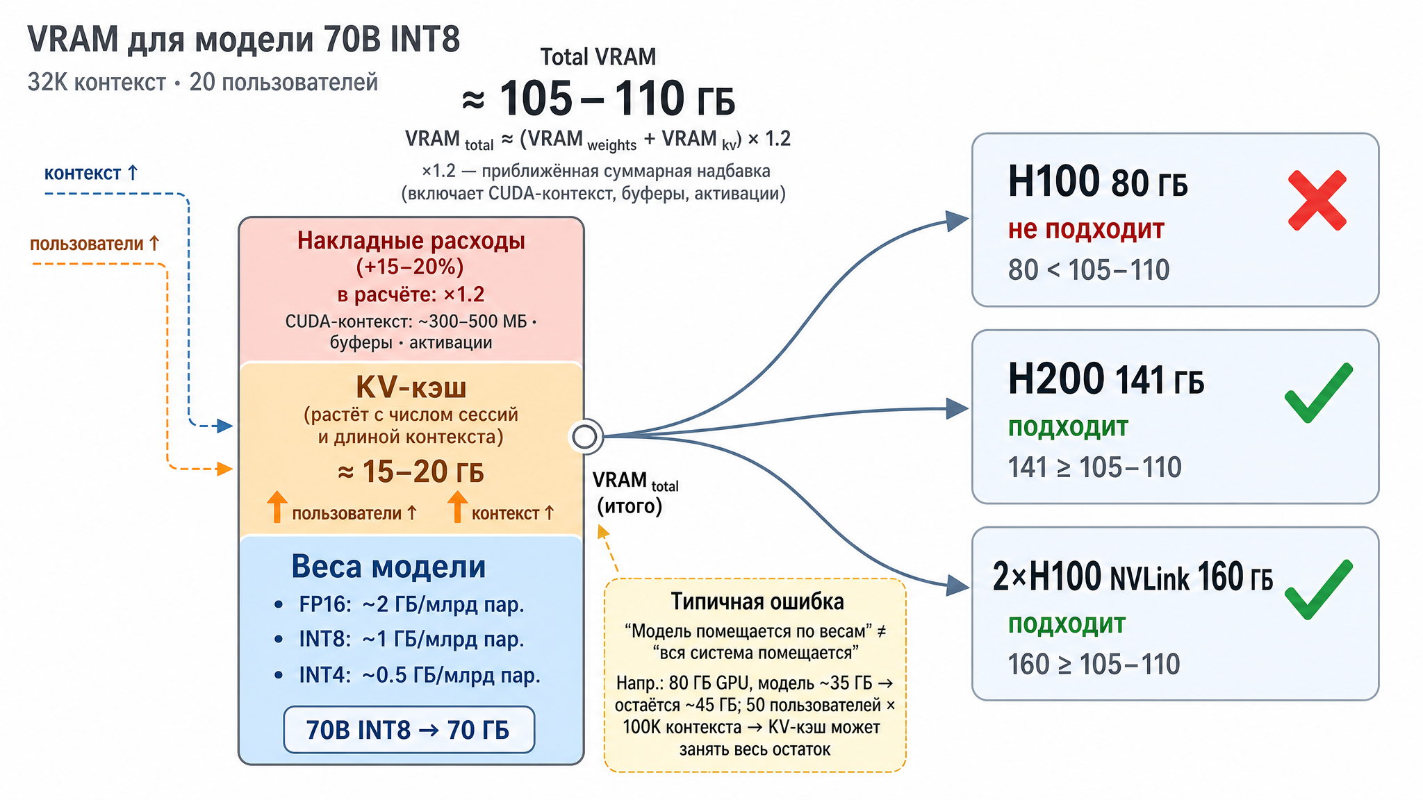
Fig. 2. GPU VRAM breakdown: model weights, KV-cache, and overhead
The MoE quirk
A special note on Mixture-of-Experts (MoE) models. I mentioned above: on each token, such a model activates only a subset of weights — which is why MoE models are fast. But there’s a non-obvious memory trap. MoE models report two parameter counts: total and active. For example, Qwen 3 235B has only 22B active; DeepSeek V4 Pro has 1.6T total with 49B active; Kimi K2 — 1T with 32B active.
The temptation is to estimate memory by active parameters: “since only 22B are active, it should fit in memory like a small model.” Obviously, no. Active parameters determine speed, but all weights must sit in memory — because any expert might be needed for the next token. The same Qwen 3 235B in FP8 is about 235 GB of weights, meaning at least two or three GPUs, even though the model runs at 22B speed. The correct takeaway: MoE saves compute, not memory.
Working through an example
Let’s put it together. Say we need a main LLM: 70B dense (non-MoE) parameters, INT8 quantization, 32K context, up to 20 concurrent users.
- Weights: 70B × 1 byte ≈ 70 GB
- KV-cache for 32K × 20 requests ≈ 15–20 GB (depends on architecture)
- Overhead ×1.2 → total around 105–110 GB
What this means for hardware: one H100 (80 GB) won’t cut it. One H200 (141 GB) works, with room to spare. Two NVLink-connected H100s also work. The choice between “one H200” and “two H100s” comes down to price and whether you need NVLink for other tasks.
How much it can handle — sizing throughput
VRAM answers “will the model fit.” Single-stream speed we’ve also covered — that’s decode and memory bandwidth. The remaining practical question: how does one card serve many users concurrently, not just one at a time.
The key technique is continuous batching, and a proper engine like vLLM does this well. The naive approach would be: collect a batch of requests, process completely, return, grab the next one — with the card sitting idle between batches. Continuous batching (via PagedAttention) works differently: requests are mixed into processing on the fly — while one request is finishing its response (decode), another just arrived and is reading its prompt (prefill). The card stays busy continuously. Compared to old engines this gives a 2–4× throughput improvement — so one card serves noticeably more users than a naive estimate would suggest.
Service quality is measured by two metrics — and they’re what you scale by. They correspond to the same two phases we covered:
- TTFT (Time To First Token) — how long the user waits before the first word of the response. Determined by the prefill phase: the model must read and process the entire prompt.
- ITL (Inter-Token Latency) — the pause between words in an ongoing response. Determined by the decode phase and, accordingly, memory bandwidth.
When planning capacity, reason like this: how many concurrent requests can the card hold at acceptable TTFT and ITL — that’s how many it can serve. The exact number only comes from benchmarking on your model and request profile, but the order of magnitude is estimated from VRAM (how many KV-caches fit) and bandwidth (is there enough speed for everyone in the batch). The more concurrent users, the larger the KV-cache and the higher the ITL. At some point the card saturates: you can keep adding requests, but there’s no point — bandwidth has hit its ceiling and latency just keeps climbing. That saturation point is what you need to find: past it, it’s time to add hardware.
Phase disaggregation — separate nodes for prefill and decode
We know that inference consists of two phases with opposite characters: prefill (prompt processing) is compute-bound, decode (response generation) is memory-bandwidth-bound. Continuous batching from the previous section runs both phases on the same card interleaved — and there’s a nasty effect hiding here.
Imagine: a card is generating responses for twenty users (decode — computationally light). Then a request comes in with a 100K-token prompt — the card needs to run a heavy prefill. While it’s busy with that, generation for everyone else freezes: their tokens aren’t being computed, the pause between words grows. This is called head-of-line blocking — one long request sits at the front of the queue and slows everyone else down. So the two phases, sharing one card, interfere with each other: prefill ruins ITL for other requests’ decode. And you can’t tune or scale them independently either — they’re glued together.
The disaggregation idea is simple: route the phases to different groups of cards. Some nodes handle only prefill, others handle only decode. A request’s journey looks like this:
- The request lands on a prefill node. It reads the prompt and computes the KV-cache — the most expensive, compute-intensive part.
- The computed KV-cache is transferred to a decode node.
- The decode node takes that cache and calmly generates the response token by token, uninterrupted.
A router orchestrates everything: accepts the request, sends it to a free prefill node, remembers where the KV-cache went, and connects the decode node.
What this gives you:
- Phases stop interfering with each other. A heavy prefill for one request no longer stalls generation for everyone else: decode nodes are busy only with generation, prefill nodes only with prompt processing.
- Each phase can be scaled independently. Many long prompts and short answers (summarization, RAG, codebase analysis) — add prefill nodes. Short queries and long answers (regular chat) — add decode nodes. Tune the pool ratio to your traffic.
- Each phase gets its own hardware and settings. Prefill likes compute power, decode likes wide memory. You can even use different cards per phase: beefier compute for prefill, fast and large memory for decode. Parallelism and batch size are tuned independently.
- TTFT and ITL are tuned separately. Before, speeding up one inevitably degraded the other — not anymore.
An important caveat: between the prefill and decode nodes you need to transfer the KV-cache, and this isn’t a short message — it’s a whole block of memory (gigabytes on a long context). So the nodes must be connected by a fast link: NVLink within a server or InfiniBand/RoCE (i.e., RDMA) between servers. If the link is slow (regular TCP Ethernet), cache transfer becomes the bottleneck — NVIDIA’s benchmarks show TTFT without RDMA jumping from ~355 ms to 10+ seconds, roughly a 40× increase (NVIDIA Dynamo documentation, Disaggregated Serving). Plus there’s additional plumbing: the router, cache transfer layer, node coordination. Takeaway: disaggregation is justified at high traffic and with fast networking; for one or two cards and modest load it’s unnecessary complexity.
Numbers from various sources to give a sense of scale:
- DistServe (research paper, OSDI 2024) — up to 7.4× more requests at the same latency requirements, or 12.6× stricter SLOs on the same hardware.
- Splitwise (Microsoft) — 2.35× throughput on the same resources.
- Mooncake (Moonshot AI, powering Kimi) — approximately +525% via a KV-cache-centric architecture.
- NVIDIA Dynamo — up to 30× on DeepSeek-R1 (GB200 NVL72 rack) and more than 2× on Llama 70B (Hopper).
- llm-d on AWS — up to +70% tokens per second as concurrent users grow.
The spread is large and depends heavily on workload, but the conclusion holds: on the right profile (especially with long prompts) disaggregation delivers multiplier gains, not percentage gains.
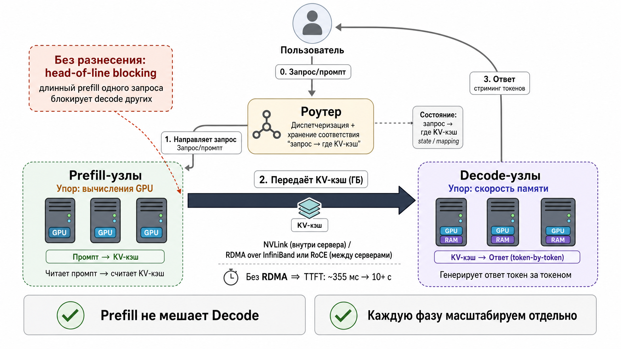
Fig. 3. Disaggregated serving architecture: prefill and decode on separate nodes
What you build this with. There are already several ready options:
- NVIDIA Dynamo — an orchestrator, meaning a layer that manages prefill/decode pools on top of regular inference engines (vLLM, SGLang, TensorRT-LLM — the engines that actually run the model). Cache transfer is handled by its NIXL library (NVIDIA Inference Transfer Library): it moves data from one card’s memory to another’s, automatically choosing the fastest available channel — NVLink, InfiniBand, etc.
- llm-d — a Kubernetes-native solution. Accepted into CNCF Sandbox in March 2026 (CNCF is the Cloud Native Computing Foundation — the organization behind Kubernetes and its ecosystem; Sandbox is the initial “incubation” maturity tier).
- vLLM — the engine itself has a built-in disaggregation mode, called disaggregated prefilling.
KV-cache transfer between nodes in all cases runs over RDMA (Remote Direct Memory Access — technology that lets one machine directly read and write another’s memory over the network, bypassing the CPU and OS; hence the low latency). On top of RDMA run transport libraries — the already-mentioned NIXL or UCX (Unified Communication X, an open communication framework from the HPC world).
Let’s walk through an example
Let’s pull everything together into an end-to-end example — go back to that AI assistant from the beginning and work it through to actual hardware and models. The client is fictional; any resemblance is coincidental: a large financial institution in a heavily regulated jurisdiction in a warm country, where by law customer data must not leave the country.
What the client wants, briefly
Not one model, but a whole platform for four use cases:
- Internal document search — Q&A over policies, regulations, and instructions, with a mandatory source citation.
- Customer support — a chat, messenger, and phone (voice) assistant that knows how to hand off to a live agent the moment it hesitates.
- Sales assistant — suggests to a manager which product to offer a customer, without straying outside compliance guardrails.
- “Talk to your data” — a natural language analyst: the user asks in plain language, the system queries the data warehouse (essentially generating SQL) and returns numbers with source attribution.
Plus cross-cutting requirements that ultimately drive the hardware decisions:
- Two working languages — English and local, with the local language having a dialect that many models handle poorly.
- Closed perimeter: external cloud APIs are out, open-weight models only, hosted in-house.
- Latency: text under 2 seconds, heavy synthesis or reports under 5, voice under 1.5.
- Load: around 1,000 concurrent text sessions, up to 100 voice sessions, up to 50 parallel analytics queries; 24/7 operation.
- Every response with a citation; everything logged; agents access data only with the permissions of the user who asked.
What drives the decisions
Let’s translate the requirements into technical implications — that’s half the architect’s job:
- “Data doesn’t leave the perimeter” → on-prem or sovereign cloud plus open-weight models. No external API possible.
- “Local language with dialect” → the model must actually support it. This immediately crosses out some popular models (examples below).
- “Voice” → a separate ASR model (speech-to-text) and dedicated cards; the main LLM doesn’t do speech recognition.
- “Talk to your data” and “sales assistant” → these are agentic tasks: the model needs to call tools and reason, not just chat smoothly.
- “Citations and source grounding” → RAG is needed: an embeddings model plus a vector database, also inside the perimeter.
- Latency and load → the VRAM and throughput calculations from the previous sections.
Model candidates and why
There’s no one model for everything — different tasks use different models, that’s normal.
- Main LLM (chat, document search, summarization): a multilingual open-weight model with long context and a clean license. A good candidate — Qwen 3 235B-A22B: Apache 2.0 license (commercial use without headaches), strong multilingualism, long context, MoE — meaning fast (only 22B active, though all 235B sit in memory — remember the MoE trap).
- Reasoning and agents (analytics, SQL generation, multi-step tasks): a model stronger at reasoning and tool use. Candidate — DeepSeek V4 Pro: MIT license, very long context, strong specifically at reasoning and tool-use — exactly what the “talk to your data” agent needs.
- Voice (speech to text): no need for a giant, just a lightweight ASR model with support for the target language — in the class of Whisper or Qwen3-ASR (around 1–2B parameters). Runs on one or two modest cards.
- Embeddings for RAG: a small multilingual embeddings model — run separately, cheap.
- Agentic “premium” — pending: there are models like Kimi K2 (strong in agentic scenarios), but it uses a “community license” with revenue and user count thresholds, not clean open-source. For a regulated bank that means — lawyers first, production second.
And separately — who didn’t make the cut and why. A strong model can be crossed out immediately for two reasons: license or language. Example: weights are closed or gated on download, or the available open versions simply don’t cover the target language — and it doesn’t matter how good the model is on benchmarks, it won’t work. Conversely: if a specialized local model exists for your specific language or dialect, keep it in mind as a way to improve quality on customer-facing channels.
How to choose a model — a short checklist
What else to look at beyond size:
- License. Apache 2.0 or MIT — take it and run. Community licenses with thresholds, gated weights (where the model seems open but can’t be downloaded freely — requires a license application and could be revoked), commercial restrictions (e.g., banned from using the model to train other models) — worth clarifying before you dig into benchmarks.
- Language and dialect. Test on your language and your texts, not the English-language leaderboard. A model that’s good on average often fails on a specific dialect.
- Agentic capability and tool use. If you have an agent (accesses tools, queries data), look specifically at the ability to call functions and maintain a multi-step plan.
- Context length. RAG and agents need a long context — otherwise documents and conversation history won’t fit.
- Multimodality. When you need to process images, audio, documents.
- Reasoning models vs. latency. These are models trained to “think out loud” first — run a long chain of intermediate reasoning before giving an answer. They’re stronger at complex tasks (math, logic, analysis) but slower and more expensive: a lot of tokens are spent on thinking before the first word of the response. So: great for analytics where you can wait, bad for voice with a 1.5-second limit.
- MoE vs. dense. MoE is faster at the same size, but all weights sit in memory (yes, I’m repeating myself).
- Ecosystem. Is the model supported in vLLM/SGLang? Are pre-built quantizations (FP8/FP4) available? Without this you spend months on infrastructure instead of shipping.
- And most importantly — your own benchmark. Collect a small set of questions with reference answers on your data and run candidates through it. Public benchmarks can be misleading for your specific task. You may also need to fine-tune the model for your domain (this usually applies to smaller models — here’s a practical example).
Sizing the hardware and sketching the deployment
Simple arithmetic — take the main LLM, Qwen 3 235B in FP8:
- Weights: 235B × 1 byte ≈ 235 GB. Multiple cards right off the bat.
- KV-cache for high concurrency (hundreds of simultaneous sessions, long context) — tens more gigabytes.
- With overhead ×1.2 → around 300+ GB just for the main LLM.
So the main LLM needs a node with multiple cards (say, 4–8 × H100/H200 SXM connected via NVLink): the model is sliced across all cards on the node — this is called tensor parallelism. The voice ASR model is small — one or two L40S cards are plenty. The embeddings model and reranker — also on modest cards. The analytics model (DeepSeek, the stronger-reasoning one) — a separate multi-card node, or the same pool if memory permits.
Important to note: this is a memory calculation. It only answers “will the model fit?” and defines the size of one pool — but it doesn’t yet say how many users that pool can handle. How many concurrent requests it holds at the required latencies is a throughput question (covered above) and is calculated separately. For now: one pool is this multi-card node, and how many such pools you need for real load we’ll figure out next.
A reasonable starting layout looks like this:
- Main LLM pool: a node with 8 × H100 SXM on NVLink, running vLLM with tensor parallelism across cards. On top — autoscaling: it automatically adds and removes model replicas as request queues and latencies grow. The ready-made stack for this is KServe and KEDA on top of Kubernetes (Kubernetes manages containers; KServe serves the model, KEDA watches load and signals when to add a replica).
- Voice pool: 1–2 cards for speech recognition. Voice is hard-constrained on latency (1.5s), so it’s kept separate so heavy text traffic doesn’t slow it down.
- Document search layer (RAG): embeddings model plus a vector database (Milvus or pgvector) on encrypted NVMe — inside the perimeter.
- Gateway and governance: PII masking, citation and policy checks before response delivery, audit log — at ingress and egress.
- At high concurrency — prefill/decode disaggregation from the previous section, so long requests don’t kill latency for everyone else.
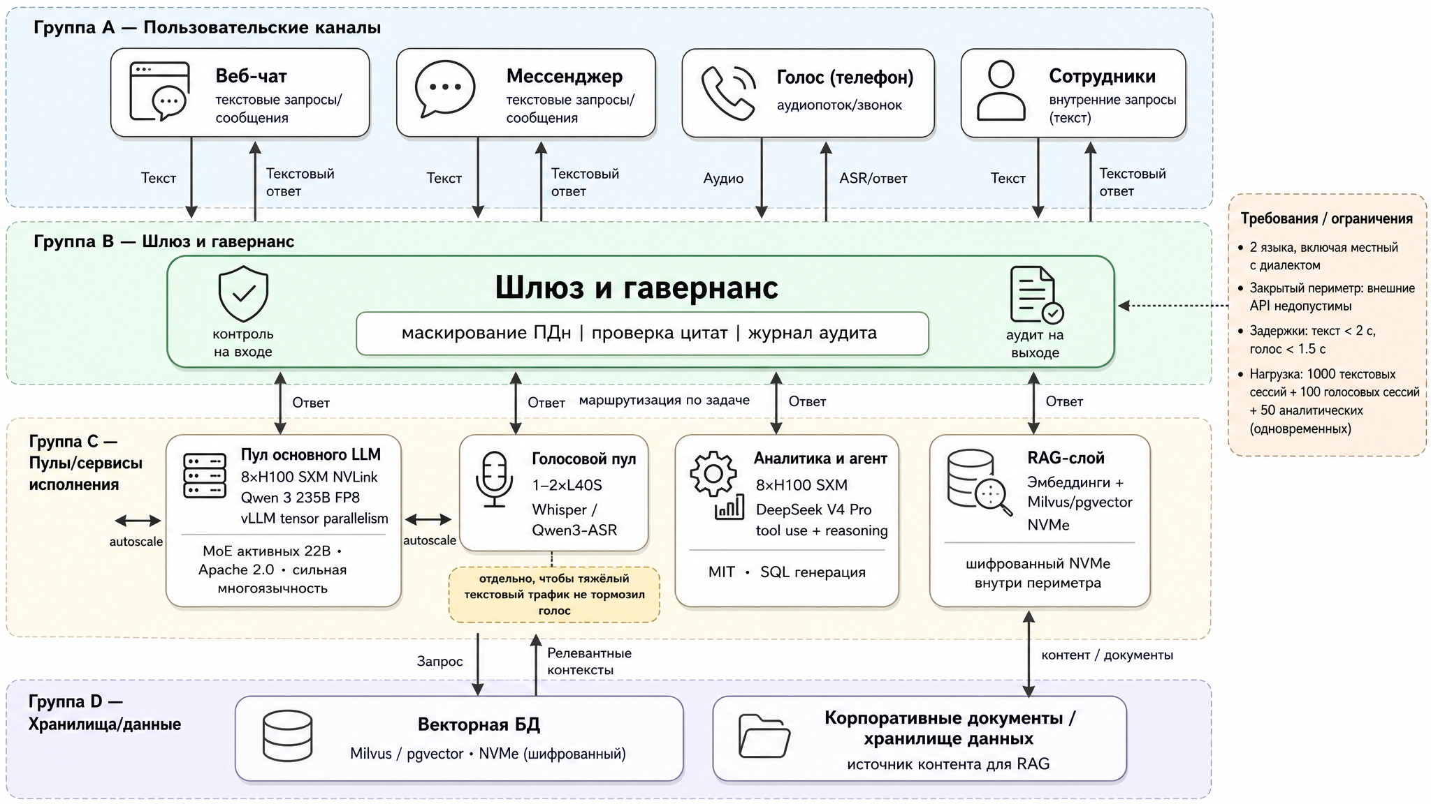
Fig. 4. Platform architecture for the financial client: model pools, gateway, and RAG layer
Where all of this physically lives — usually three options, and the choice comes down to budget, timelines, and the regulator’s risk appetite:
- Fully on-prem. Your own data center, starting pod of ~8 × H100 (tens of kilowatts and serious electrical infrastructure). Maximum protection: data physically goes nowhere. Downside — large capex, long GPU delivery times, and 2–3 people needed for operations.
- Hybrid. Sensitive workloads (voice, PII, customer index) — on a small on-prem footprint (2 × H100 or 4 × L40S is enough), with heavy anonymized inference in a sovereign cloud within the country. At the boundary — a tokenizing gateway: it replaces PII with anonymized tokens before the request leaves for the cloud. Usually the best balance: lower capex, faster start, perimeter intact.
- Turnkey appliance. A ready-made box (DGX BasePOD, Dell AI Factory) — if you don’t have an infrastructure team but do have budget. More on this shortly.
For a regulated financial client, hybrid wins in practice most often: strong protection (raw data doesn’t leave the perimeter), moderate capex, and the ability to start development in the cloud portion while the on-prem hardware is still in transit. Fully on-prem is chosen when the risk committee won’t accept any external dependency whatsoever — not even sovereign.
How many users it handles — and how to scale
Remember that the model itself has no concept of “users” or “sessions”: it processes individual requests and forgets everything between them — each request arrives with its full context. A dialogue in an application is just a sequence of independent requests from the model’s perspective. So hardware is sized not by people or conversations, but by requests “in flight” — how many requests the model is generating at this exact moment. “5,000 employees” doesn’t mean “5,000 simultaneous requests”: most are silent at any given moment. What we need is peak concurrent load — how many requests are in flight during the worst minute of the day.
Rough estimate, step by step:
- Total users. Say 5,000 internal employees.
- How many are active at peak. For an internal tool this is typically 10–20% online simultaneously — let’s take 15%, about 750 people. I’ve seen call center utilization stats somewhere with roughly these numbers.
- How many of those are waiting for a response right now. A person reads the response, thinks, types — the actual generation takes a small fraction of their time. If an active user has a request “in flight” about 5% of the time, then out of 750 online, 30–40 responses are being generated simultaneously. Even with a 3× safety factor — that’s about a hundred concurrent requests, not five thousand.
- How many a single pool can hold. Comes from benchmarking (see “How much it can handle”): say a node with 8 × H100 at acceptable latencies handles N concurrent requests. Let’s say N ≈ 150.
- Divide and round up, adding a margin for node failure: you need “concurrent ÷ N” rounded up, plus one more pool in reserve.
The counterintuitive result: 5,000 internal employees in regular chat mode is only about a hundred in-flight requests — one main LLM pool plus a reserve pool. The relationship between headcount and hardware is nonlinear. Most “users” are silent at any moment, so counting by heads is meaningless — count in-flight requests.
But more important than the number itself is this: the same number of people produces completely different loads depending on what they’re doing. The same 5,000 people:
- Regular chat and document search: short queries, a couple seconds of generation, long pauses to read. Tiny in-flight fraction → about a hundred concurrent requests → 1–2 pools.
- Agents and analytics: each request runs a long time — the model runs a multi-step plan, queries data, produces long answers. In-flight fraction jumps several times → hundreds of concurrent requests → 4–8 pools for the same 5,000 people.
- Long context: bloats the KV-cache, and one card handles fewer simultaneous requests (that N drops) → more pools needed.
Key points on scaling:
- Scale out by replicating the model. Model size is determined by task quality requirements; number of users is served by number of replicas.
- Scale automatically to peak. Spin up extra replicas during peak hours and scale down during quiet periods (but remember the cold start cost of large models — keep a warm reserve).
- Disaggregate prefill and decode at high concurrency — so long requests don’t eat everyone else’s latency budget.
- Compress to fit more. INT4 model quantization and KV-cache quantization free up memory — one card fits more concurrent requests.
- Cache context (prompt caching) for agents and repeated prompts — removes the bulk of the prefill load.
- Benchmark on your profile. An internal tool and a public chatbot produce completely different user-to-concurrency ratios.
DGX SuperPOD — an interesting example
Disclaimer upfront: I haven’t personally had the chance to work with one of these — so this is still theoretical analysis on my part.
NVIDIA has this thing called DGX SuperPOD. It’s essentially a turnkey AI supercomputer at data center scale: NVIDIA ships and assembles an entire cluster of DGX nodes interconnected by high-speed InfiniBand, with shared storage and management software.
A DGX node is a factory-built server from NVIDIA itself: a pre-assembled chassis with 8 accelerators, CPUs, built-in NVLink, and NICs (in the GB200 generation, a “node” is an entire NVL72 rack with 72 GPUs). It’s essentially the same inference node described above, just in a vendor-assembled form factor.
How it’s structured. The cluster is assembled from identical building blocks — scalable units (SU). In the GB200 version, one SU consists of 8 DGX GB200 NVL72 racks and consumes around 1.2 MW. From these blocks, configurations are built up to 128+ racks — thousands of GPUs in a single network. Think of it as a construction kit. You start with one or two blocks, then grow the cluster by snapping on more SUs — identical ones. Growth happens in known-size, known-power, known-performance cubes, not card by card.
What it’s for. SuperPOD is designed for two things: training trillion-parameter giants and inference at factory scale — when you’re serving millions of users or running frontier models at the limit. A different scale entirely.
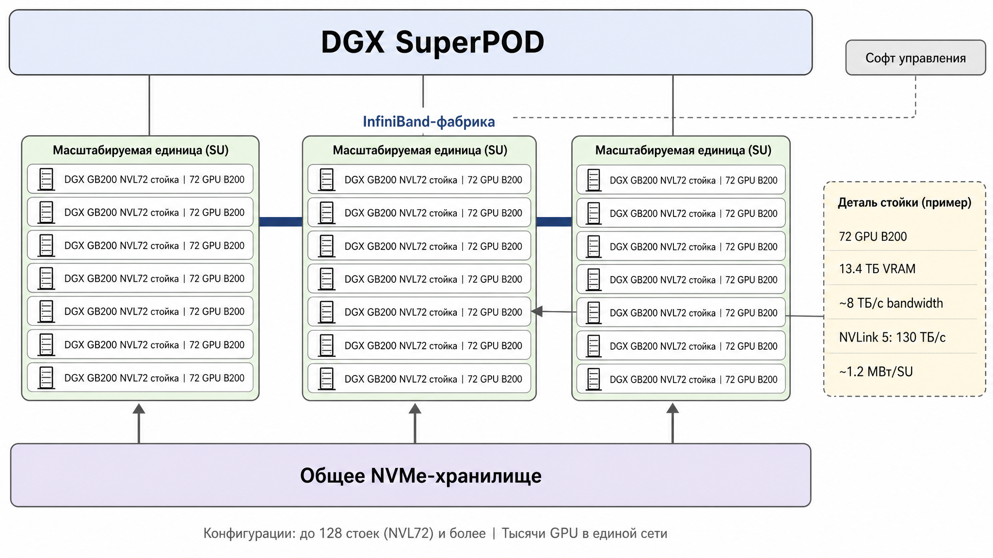
Fig. 5. DGX SuperPOD architecture: scalable units (SU), InfiniBand fabric, and shared storage
What it gives you:
- Scale from day one. Thousands of GPUs work as a single cluster with predictable performance — assembling this yourself from individual cards is nearly impossible.
- Grows like a construction kit. The reference architecture pre-calculates network, storage, and power for growth, so adding another SU is snapping in a known cube, not redesigning the whole architecture.
- Fast start. This is a tested, proven reference configuration: NVIDIA ships, installs, configures network and software. Months of integration become weeks.
- Network without bottlenecks. InfiniBand is designed so any pair of nodes communicate at full speed; the whole point of the architecture is that distributed work across thousands of cards doesn’t get strangled by the network.
- Support and software included. Cluster management, job scheduler, monitoring — all pre-assembled and vendor-supported.
Downsides:
- Price and power are not for midsize businesses. One DGX node with 8 accelerators costs around $400–500K (Blackwell generation is even more), and a full SuperPOD runs into tens of millions: Texas A&M bought a 760-GPU SuperPOD for $45M. On power — ~1.2 MW per SU per NVIDIA’s reference architecture. You need a dedicated Tier 3 data center with liquid cooling, not a server room.
- Fixed configuration and long lead times. It’s a standard design with a waiting list; flexibility is limited, delivery time is quarters.
- NVIDIA ecosystem lock-in. Hardware, networking, and software — all one vendor.